Boundary Layer Velocity Profile Ekman Layer or Outer

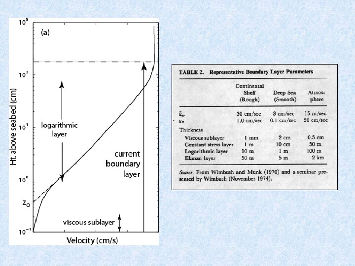
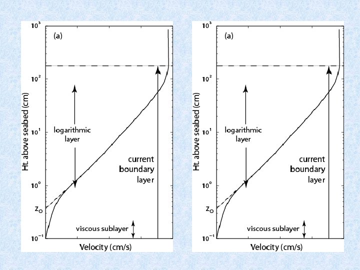
Boundary Layer Velocity Profile Ekman Layer, or Outer region z (velocity defect layer) Logarithmic turbulent zone Buffer zone Viscous sublayer ū

But first. . a definition:

1. Viscous Sublayer - velocities are low, shear stress controlled by molecular processes As in the plate example, laminar flow dominates, Put in terms of u* integrating, boundary conditions,

When do we see a viscous sublayer? v = f (u*, , ks) where ks == characteristic height of bed roughness Re: R* > 70 rough turbulent no viscous sublayer R* < 5 smooth turbulent yes, viscous sublayer

2. Log Layer: Turbulent case, Az is NOT constant in z Az is a property of the flow, not just the fluid To describe the velocity profile we need to develop a profile of Az. Mixing Length formulation Prandtl (1925) which is a qualitative argument discussed in more detail “Boundary Layer Analysis” by Shetz, 1993 Assume that water masses act independently over a distance, l Within l a change in momentum causes a fluctuation to adjacent fluid parcels.

At l, Make assumption of isotropic turbulence: |u’| ~ |v’| ~ |w’| Therefore, |u’| ~ |w’| ~ Through the Reynolds Stress formulation, Prandtl Mixing Length Formulation

Von Karmen (1930) hypothesized that close to a boundary, the turbulent exchange is related to distance from the boundary. l z l = Kz where K is a universal turbulent momentum exchange coefficient == von Karmen’s constant. K has been found to be 0. 41 Near the bed, in terms of u*

Solving for the velocity profile: ln z ū Intercept, b, depends on roughness of the bed - f (R*)

Rename b, based on boundary condition: z = zo at ū = 0 Karmen-Prandtl Eq. or Law of the Wall

Hydraulic Roughness Length, zo zo is the vertical intercept at which ūz = 0 zo = f ( viscous sublayer, grain roughness, ripples & other bedforms, stratification) This leads to two forms of the Karmen-Prandtl Equation 1) with viscous sublayer HSF 2) without viscous sublayer HRF

Can evaluate which case to use with R* where ks == roughness length scale in glued sand, pipe flow experiments ks = D in real seabeds with no bedforms, ks = D 75 in bedforms, characteristic bedform scale ks ~ height of ripples

1. Hydraulically Smooth Flow (HSF) ** boundary layer is turbulent, but there is a viscous sublayer zo is a fraction of the viscous sublayer thickness: Karmen-Prandtl equation becomes: For turbulent flow over a hydraulically smooth boundary

2. Hydraulically Rough Flow (HRF) zo is a function of the roughness elements ** no viscous sublayer Nikaradze pipe flow experiments: Karmen-Prandtl equation becomes: For turbulent flow over a hydraulically rough boundary with no bedforms, no stratification, etc.

Notes on zo in HRF Grain Roughness: Nikuradze (1930 s) - glued sand grains on pipe flow zo = D/30 Kamphius (1974) - channel flow experiments zo = D/15 Bedforms: Wooding (1973) where H is the ripple height and is the ripple wavelength Suspended Sediment: Smith (1977) zo = f (excess shear stress, and zo from ripples)

3. Hydraulically Transitional Flow (HTF) zo is both fraction of the viscous sublayer thickness and a function of bed roughness. Karmen-Prandtl equation is defined as:

Bed Roughness is never well known or characterized, but fortunately not necessary to determine u* If you only have one velocity measurement (at a single elevation), use the formulations above. If you can avoid it. . do so. With multiple velocity measurements, use the “Law of the Wall” to get u* ln z ūz

To determine b (or u* ) from a velocity profile: 1. Fit line to data 2. Find slope 3. Evaluate