Boundary conditions for SU2 YangMills on Ad S

Boundary conditions for SU(2) Yang-Mills on Ad. S 4 Jae-Hyuk Oh At ISM meeting in Puri, 2012. 20. Dileep P. Jatkar and Jae-Hyuk Oh, Based on ar. Xiv: 1203. 2106

Program • 1. Alternative quantization for massive scalar and U(1) fields. • 2. Its extension to SU(2) Yang-Mills and interesting boundary actions. • 3. “Approximate” electric-magnetic duality. • 4. Yang-Mills instanton in Ad. S and its boundary condition.

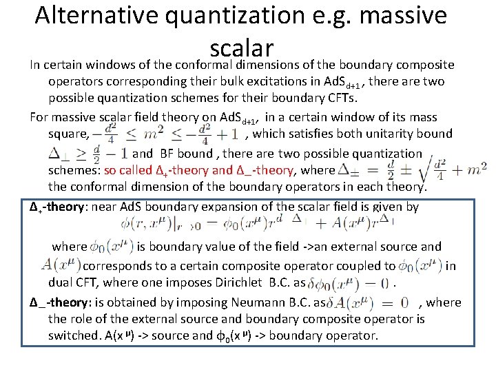
Alternative quantization e. g. massive scalar In certain windows of the conformal dimensions of the boundary composite operators corresponding their bulk excitations in Ad. Sd+1 , there are two possible quantization schemes for their boundary CFTs. For massive scalar field theory on Ad. Sd+1, in a certain window of its mass square, , which satisfies both unitarity bound and BF bound , there are two possible quantization schemes: so called Δ+-theory and Δ—-theory, where the conformal dimension of the boundary operators in each theory. Δ+-theory: near Ad. S boundary expansion of the scalar field is given by where is boundary value of the field ->an external source and corresponds to a certain composite operator coupled to in dual CFT, where one imposes Dirichlet B. C. as . Δ—-theory: is obtained by imposing Neumann B. C. as , where the role of the external source and boundary composite operator is switched. A(x μ) -> source and φ0(x μ) -> boundary operator.

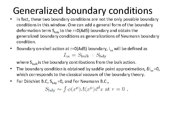
Generalized boundary conditions • In fact, these two boundary conditions are not the only possible boundary conditions in this window. One can add a general form of the boundary deformation term Sbdy to the r=0(Ad. S) boundary and obtain the generalized boundary conditions as generalizations of Neumann boundary condition. • Boundary on-shell action at r=0(Ad. S) boundary, Ios will be defined as where Sbulk is the boundary contributions from the bulk action. • The boundary condition is obtained by saddle point approximation, δIos =0, which corresponds to the classical vacuum of the boundary theory. • For Dirichlet B. C, Sbdy =0, and For Neumann B. C. , .

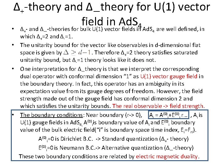
Δ+-theory and Δ—theory for U(1) vector field in Ad. S 4 • Δ - and Δ -theories for bulk U(1) vector fields in Ad. S are well defined, in + — 4 which Δ+=2 and Δ-=1. • The unitarity bound for the vector like observables in d-dimensional flat space is given by . Therefore Δ+=2 theory satisfies saturated unitarity bound, but Δ-=1 theory looks like it does not. • One interpretation for Δ—theory is that we interpret the corresponding dual operator with conformal dimension “ 1” as U(1) vector gauge field in the boundary theory. In fact, this operator has an ambiguity in its expectation value from its gauge degrees of freedom. However, the field strength made out of the gauge field has conformal dimension 2 and which satisfies the unitarity bounds. The real observable -> field strength. • The boundary conditions: Near boundary (r-> 0), Ai = A(0)i+E(0)i r… , Ai is U(1) gauge fields in Ad. S 4, A(0)iis boundary value of Ai and E(0)i boundary value of the bulk electric field(“i” is boundary space time index, Ei=Fri). A(0)i=0 is Dirichlet B. C. -> Standard quantization (Δ+- theory) E(0)i=0 is Neumann B. C. -> Alternative quantization (Δ—-theory) These two boundary conditions are related by electric magnetic duality.

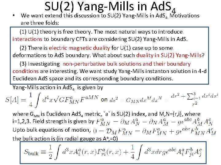
SU(2) Yang-Mills in Ad. S 4 • We want extend this discussion to SU(2) Yang-Mills in Ad. S 4. Motivations are three folds: (1) U(1) theory is free theory. The most natural ways to introduce interactions to boundary CFTs are considering SU(2) Yang-Mills in Ad. S. (2) There is electric magnetic duality for U(1) case up to some deformations to Ad. S boundary. What about such duality in SU(2) Yang-Mills? (3) Investigating non-perturbative bulk solutions and their boundary conditions are interesting. We want study Yang-Mills instanton solution in 4 -d Euclidean Ad. S space and its corresponding boundary conditions. Yang-Mills action in Ad. S 4 is given by where GMN is Euclidean Ad. S 4 metric, `a` is SU(2) index, and M, N={r, i}, where i=1, 2, 3. Field strength is given by Upto bulk equations of motion, the bulk action is (in radial gauge as Aar=0)

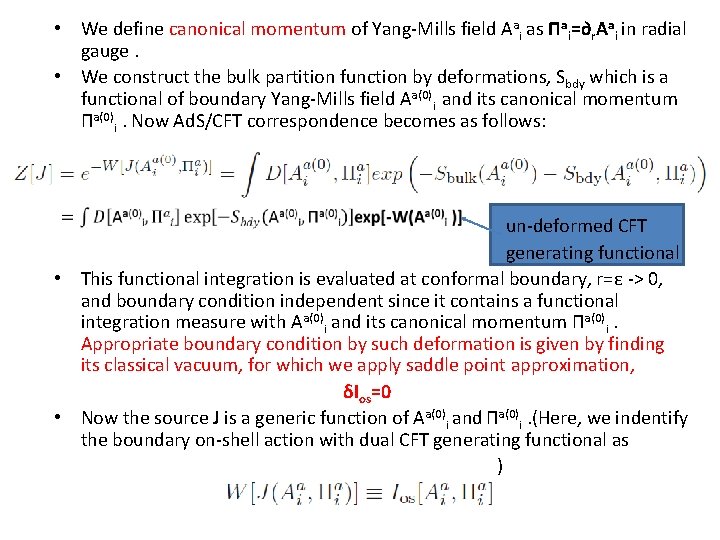
• We define canonical momentum of Yang-Mills field Aai as Πai=∂r. Aai in radial gauge. • We construct the bulk partition function by deformations, Sbdy which is a functional of boundary Yang-Mills field Aa(0)i and its canonical momentum Πa(0)i. Now Ad. S/CFT correspondence becomes as follows: un-deformed CFT generating functional • This functional integration is evaluated at conformal boundary, r=ε -> 0, and boundary condition independent since it contains a functional integration measure with Aa(0)i and its canonical momentum Πa(0)i. Appropriate boundary condition by such deformation is given by finding its classical vacuum, for which we apply saddle point approximation, δIos=0 • Now the source J is a generic function of Aa(0)i and Πa(0)i. (Here, we indentify the boundary on-shell action with dual CFT generating functional as )

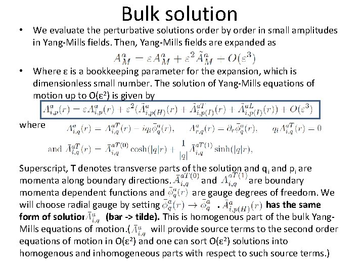
Bulk solution • We evaluate the perturbative solutions order by order in small amplitudes in Yang-Mills fields. Then, Yang-Mills fields are expanded as • Where ε is a bookkeeping parameter for the expansion, which is dimensionless small number. The solution of Yang-Mills equations of motion up to O(ε 2) is given by where Superscript, T denotes transverse parts of the solution and qi and pi are momenta along boundary directions. and are boundary momenta dependent functions and are gauge degrees of freedom. We will choose radial gauge by setting . has the same form of solution (bar -> tilde). This is homogenous part of the bulk Yang. Mills equations of motion. ( will provide source terms to the second order equations of motion in O(ε 2) and one can sort O(ε 2) solutions into homogenous and inhomogeneous parts with respect to such source terms. )

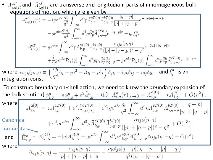
• and are transverse and longitudianl parts of inhomogeneous bulk equations of motion, which are given by where and is an integration const. To construct boundary on-shell action, we need to know the boundary expansion of the bulk solution( ): , where Canonical momenta and = , where

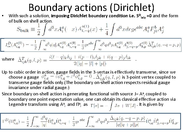
• Boundary actions (Dirichlet) With such a solution, imposing Dirichlet boundary condition i. e. SDbdy =0 and the form of bulk on shell action, where . Up to cubic order in action, gauge fields in the 3 -vertax is effectively transverse, since we choose a gauge is 3 -point vertex coupled to transverse gauge fields only. (The boundary on-shell action respects residual gauge invariance under radial gauge. ) Since boundary on-shell action is generating functional with source J= Aai coupled to boundary one point expectation value, one can obtain its classical effective action via Legendre transform using Aai and Πai as . It is given by

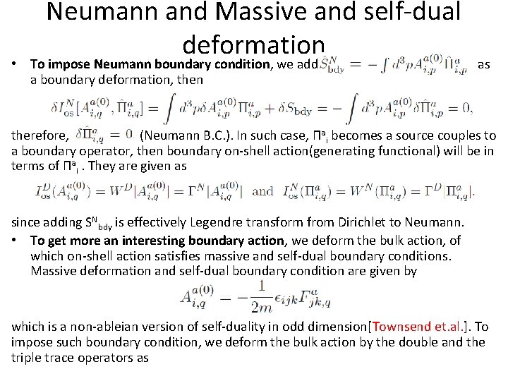
Neumann and Massive and self-dual deformation • To impose Neumann boundary condition, we add as a boundary deformation, then therefore, (Neumann B. C. ). In such case, Πai becomes a source couples to a boundary operator, then boundary on-shell action(generating functional) will be in terms of Πai. They are given as since adding SNbdy is effectively Legendre transform from Dirichlet to Neumann. • To get more an interesting boundary action, we deform the bulk action, of which on-shell action satisfies massive and self-dual boundary conditions. Massive deformation and self-dual boundary condition are given by which is a non-ableian version of self-duality in odd dimension[Townsend et. al. ]. To impose such boundary condition, we deform the bulk action by the double and the triple trace operators as

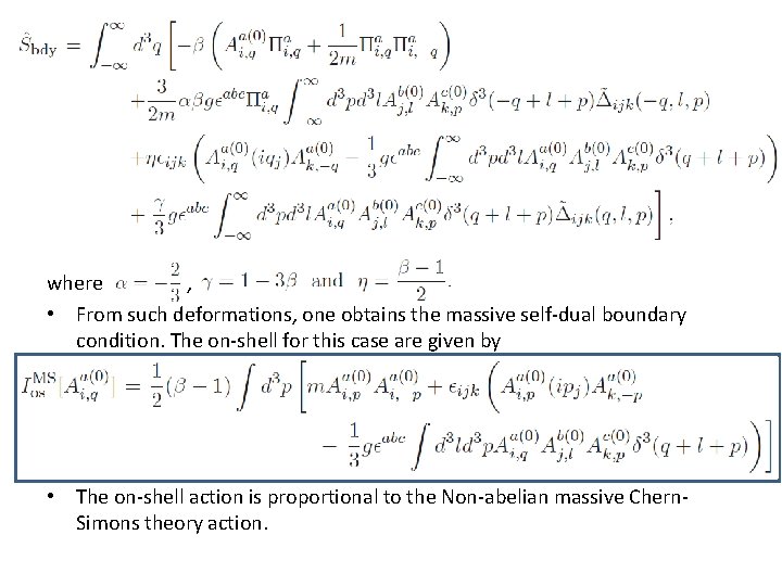
where , • From such deformations, one obtains the massive self-dual boundary condition. The on-shell for this case are given by • The on-shell action is proportional to the Non-abelian massive Chern. Simons theory action.

• “Approximate” electric magnetic duality in SU(2) Yang-Mills. It is well-known fact that electric-magnetic duality cannot be demonstrated for non-Abelian gauge fields theories. Exchanging E and B fields is still possible in these theories but the real problem is if such transformations are canonical or not. It is shown that these are not canonical transformations for the non-Ableian cases by Deser et. al. long ago. • Recently, however, it is suggested that electric magnetic duality is possible to be embodied for SU(2) gauge theory when Yang-Mills action is truncated up to cubic order interactions, at least for a particular gauge(transverse gauge). This duality is somewhat “approximate”. The meaning of “approximate” is the following: Deser et. al. have constructed an infinitesimal canonical transformation which is a natural extension of U(1) duality by retaining Yang-Mills cubic interactions only. • However, this is not precisely EM duality transform since infinitesimal changes of electric fields are not proportional to magnetic fields. Therefore, “approximate” duality only states that there exist a canonical transformation which is a natural extension of infinitesimal U(1) duality transform. • The difference between 4 -d flat and Ad. S 4 space is their boundaries. EM duality is not a symmetry of Lagrangian and there will be total derivative terms in the transformed action. In flat space, one can remove these terms since he/she can assume that the gauge fields sufficiently die off at the space time infinity. However, in Ad. S space, there is Ad. S boundary at r=0. Therefore, we need to count boundary terms at r=0 properly.

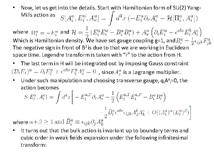
• Now, let us get into the details. Start with Hamiltonian form of SU(2) Yang. Mills action as where and Which is Hamiltonian density. We have set gauge coupling g=1, and The negative sign in front of B 2 is due to that we are working in Euclidean space time. Legendre transform is taken with “r” to the action from H. • The last term in H will be integrated out by imposing Gauss constraint , since is a Lagrange multiplier. • Under such manipulation and choosing transverse gauge, qi. Aai=0, the action becomes where • It turns out that the bulk action is invariant up to boundary terms and cubic order in weak fields expansion under the following infinitesimal transform:

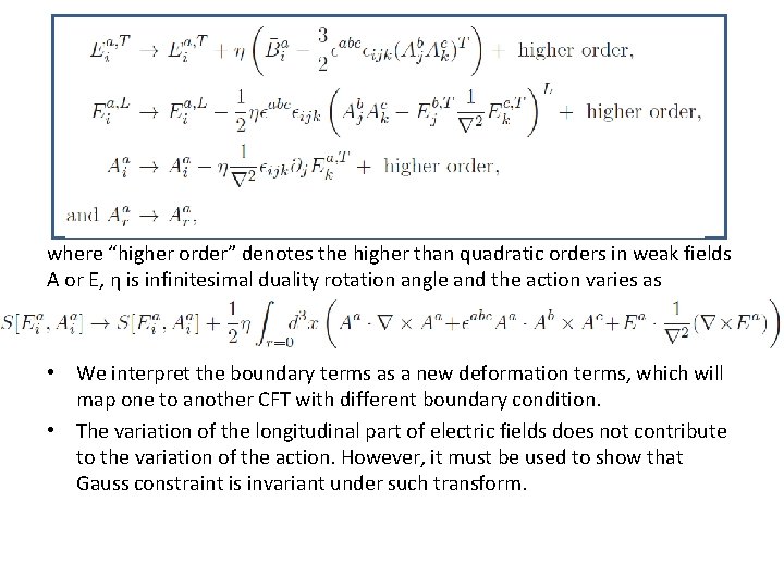
where “higher order” denotes the higher than quadratic orders in weak fields A or E, η is infinitesimal duality rotation angle and the action varies as • We interpret the boundary terms as a new deformation terms, which will map one to another CFT with different boundary condition. • The variation of the longitudinal part of electric fields does not contribute to the variation of the action. However, it must be used to show that Gauss constraint is invariant under such transform.

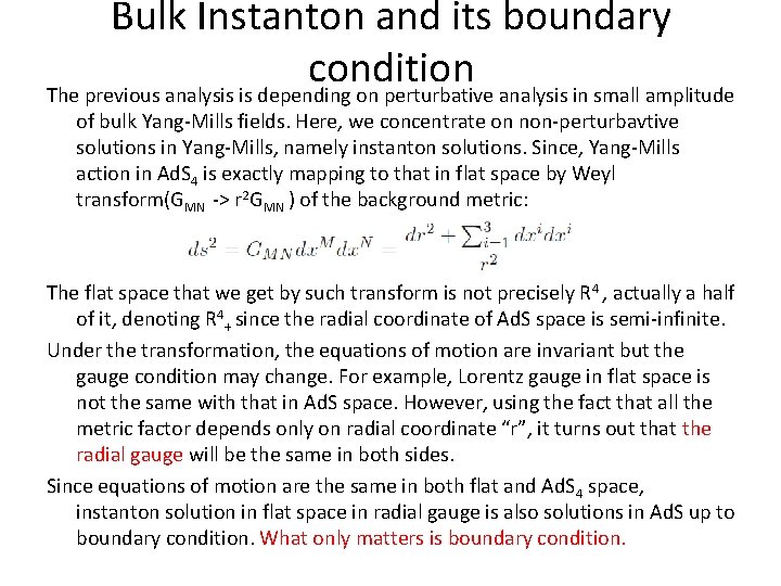
Bulk Instanton and its boundary condition The previous analysis is depending on perturbative analysis in small amplitude of bulk Yang-Mills fields. Here, we concentrate on non-perturbavtive solutions in Yang-Mills, namely instanton solutions. Since, Yang-Mills action in Ad. S 4 is exactly mapping to that in flat space by Weyl transform(GMN -> r 2 GMN ) of the background metric: The flat space that we get by such transform is not precisely R 4 , actually a half of it, denoting R 4+ since the radial coordinate of Ad. S space is semi-infinite. Under the transformation, the equations of motion are invariant but the gauge condition may change. For example, Lorentz gauge in flat space is not the same with that in Ad. S space. However, using the fact that all the metric factor depends only on radial coordinate “r”, it turns out that the radial gauge will be the same in both sides. Since equations of motion are the same in both flat and Ad. S 4 space, instanton solution in flat space in radial gauge is also solutions in Ad. S up to boundary condition. What only matters is boundary condition.

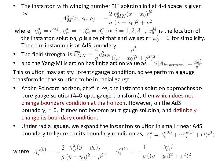
• The instanton with winding number “ 1” solution in flat 4 -d space is given by where , is the location of the instanton solution, ρ is size of that and we set r= for simplicity. Then the instanton is at Ad. S boundary. • The field strength is , • and the Yang-Mills action has finite action value as This solution may satisfy Lorentz gauge condition, so we perform a gauge transform for the solution to be in radial gauge. • At the Poincare horizon, at x 4=r=∞, the instanton solution approaches to pure gauge solution(A=0 upto gauge transform), then which does not change boundary condition at the horizon. However, on the Ad. S boundary, r=0, it does not become pure gauge solution, and definitely change its boundary condition. • Under radial gauge, we expand the instanton solution in small r near Ad. S boundary to figure our its boundary condition as, where

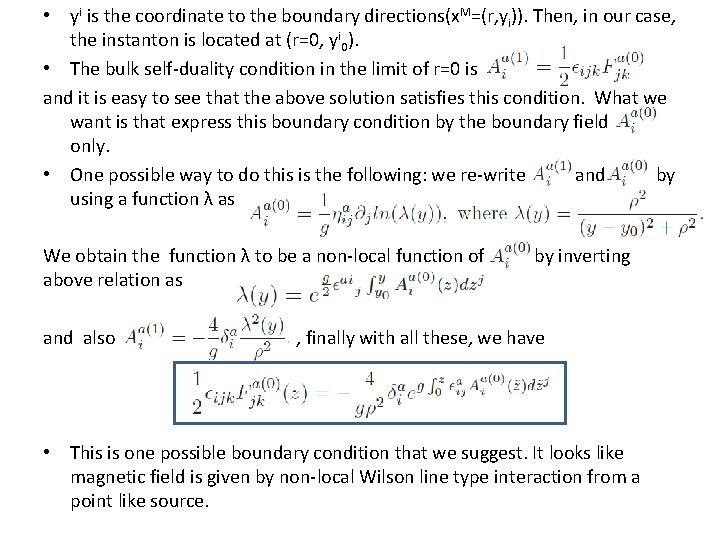
• yi is the coordinate to the boundary directions(x. M=(r, yi)). Then, in our case, the instanton is located at (r=0, yi 0). • The bulk self-duality condition in the limit of r=0 is and it is easy to see that the above solution satisfies this condition. What we want is that express this boundary condition by the boundary field only. • One possible way to do this is the following: we re-write and by using a function λ as We obtain the function λ to be a non-local function of by inverting above relation as and also , finally with all these, we have • This is one possible boundary condition that we suggest. It looks like magnetic field is given by non-local Wilson line type interaction from a point like source.

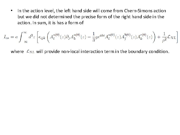
• In the action level, the left hand side will come from Chern-Simons action but we did not determined the precise form of the right hand side in the action. In sum, it is has a form of where will provide non-local interaction term in the boundary condition.

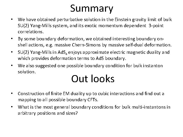
Summary • We have obtained perturbative solution in the Einstein gravity limit of bulk SU(2) Yang-Mills system, and its exotic momentum dependent 3 -point correlations. • By some boundary deformation, we obtained interesting boundary onshell actions, e. g. massive Chern-Simons by massive self-dual deformation. • SU(2) Yang-Mills in Ad. S 4 enjoys approximate electric magnetic duality and which provides deformation terms to Ad. S boundary. • We also suggested one possible boundary condition for bulk instanton solution. Out looks • Construction of finite EM duality up to cubic interactions and find out a mapping to all possible boundary CFTs. • What is the most general boundary conditions for bulk multi-instantons in arbitrary positions and sizes?