Boolean Methods for Multilevel Logic Synthesis Giovanni De

Boolean Methods for Multi-level Logic Synthesis Giovanni De Micheli Integrated Systems Laboratory This presentation can be used for non-commercial purposes as long as this note and the copyright footers are not removed © Giovanni De Micheli – All rights reserved

Module 1 u Objectives s What are Boolean methods s How to compute don’t care conditions t t s Controllability Observability Boolean transformations (c) Giovanni De Micheli 2

Boolean methods u Exploit Boolean properties of logic functions u Use don’t care conditions u More complex algorithms s Potentially better solutions s Harder to reverse the transformations u Used within most synthesis tools (c) Giovanni De Micheli 3

External don’t care conditions u Controllability don’t care set CDCin s Input patterns never produced by the environment at the network’s input u Observability don’t care set ODCout s Input patterns representing conditions when an output is not observed by the environment s Relative to each output s Vector notation (c) Giovanni De Micheli 4

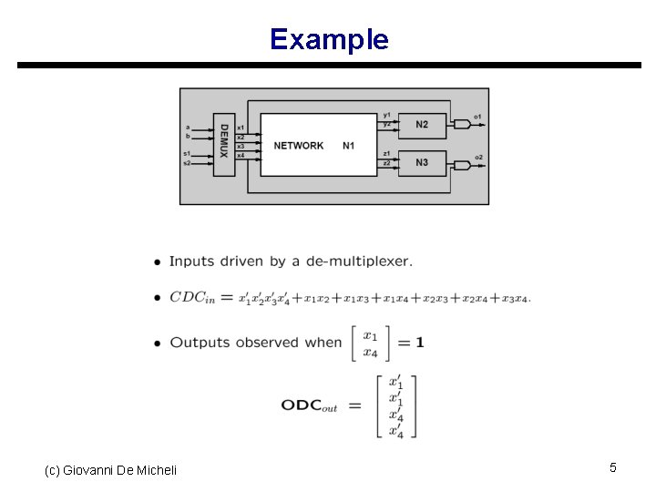
Example (c) Giovanni De Micheli 5

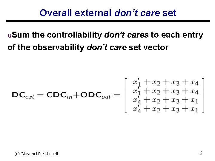
Overall external don’t care set u. Sum the controllability don’t cares to each entry of the observability don’t care set vector (c) Giovanni De Micheli 6

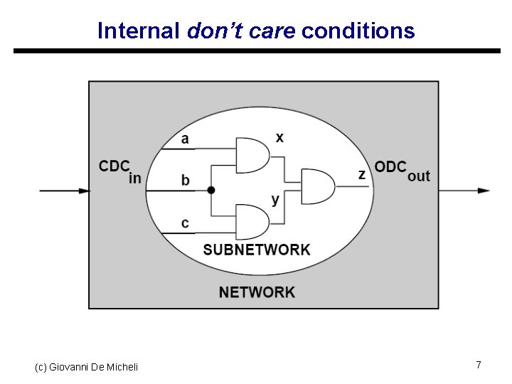
Internal don’t care conditions (c) Giovanni De Micheli 7

Internal don’t care conditions u Induced by the network structure u Controllability don’t care conditions: s Patterns never produced at the inputs of a subnetwork u Observability don’t care conditions s Patterns such that the outputs of a sub-network are not observed (c) Giovanni De Micheli 8

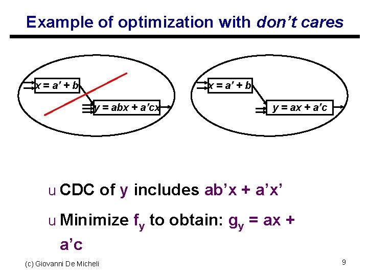
Example of optimization with don’t cares x = a’ + b y = abx + a’cx y = ax + a’c u CDC of y includes ab’x + a’x’ u Minimize fy to obtain: gy = ax + a’c (c) Giovanni De Micheli 9

Satisfiability don’t care conditions u Invariant of the network: x = fx → x ≠ fx SDC u SDC = ∑all internal nodes x fx u Useful to compute controllability don't cares (c) Giovanni De Micheli 10

CDC Computation u Method 1: Network traversal algorithm s Consider initial CDC = CDCin at the primary inputs s Consider different cutsets moving through the network from inputs to outputs s As the cutset moves forward t t Consider SDC contribution of the newly considered block Remove unneeded variables by consensus (c) Giovanni De Micheli 11

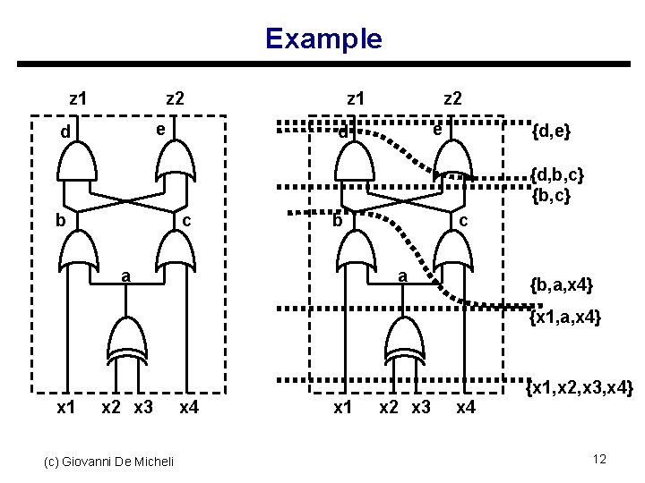
Example z 1 z 2 e d {d, e} {d, b, c} {b, c} b c b a c a {b, a, x 4} {x 1, a, x 4} x 1 x 2 x 3 (c) Giovanni De Micheli x 4 x 1 x 2 x 3 x 4 {x 1, x 2, x 3, x 4} 12

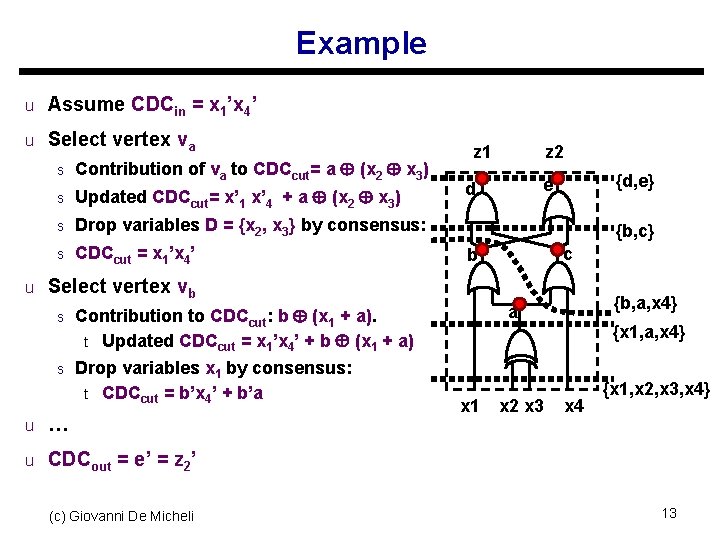
Example u Assume CDCin = x 1’x 4’ u Select vertex va s Contribution of va to CDCcut= a (x 2 x 3) s Updated CDCcut= x’ 1 x’ 4 + a (x 2 x 3) s Drop variables D = {x 2, x 3} by consensus: s CDCcut = x 1’x 4’ z 1 z 2 {d, e} e d {b, c} c b u Select vertex vb s Contribution to CDCcut: b (x 1 + a). t Updated CDCcut = x 1’x 4’ + b (x 1 + a) s Drop variables x 1 by consensus: t CDCcut = b’x 4’ + b’a u … {b, a, x 4} a x 1 x 2 x 3 {x 1, a, x 4} x 4 {x 1, x 2, x 3, x 4} u CDCout = e’ = z 2’ (c) Giovanni De Micheli 13

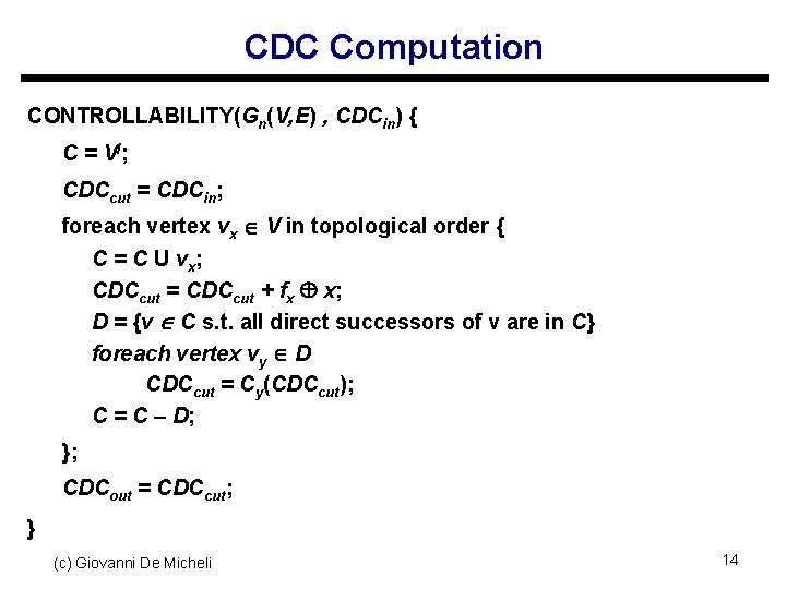
CDC Computation CONTROLLABILITY(Gn(V, E) , CDCin) { C = VI; CDCcut = CDCin; foreach vertex vx V in topological order { C = C U vx ; CDCcut = CDCcut + fx x; D = {v C s. t. all direct successors of v are in C} foreach vertex vy D CDCcut = Cy(CDCcut); C = C – D; }; CDCout = CDCcut; } (c) Giovanni De Micheli 14

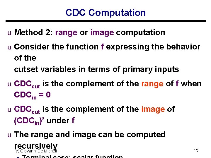
CDC Computation u Method 2: range or image computation u Consider the function f expressing the behavior of the cutset variables in terms of primary inputs u CDCcut is the complement of the range of f when CDCin = 0 u CDCcut is the complement of the image of (CDCin)’ under f u The range and image can be computed recursively (c) Giovanni De Micheli 15

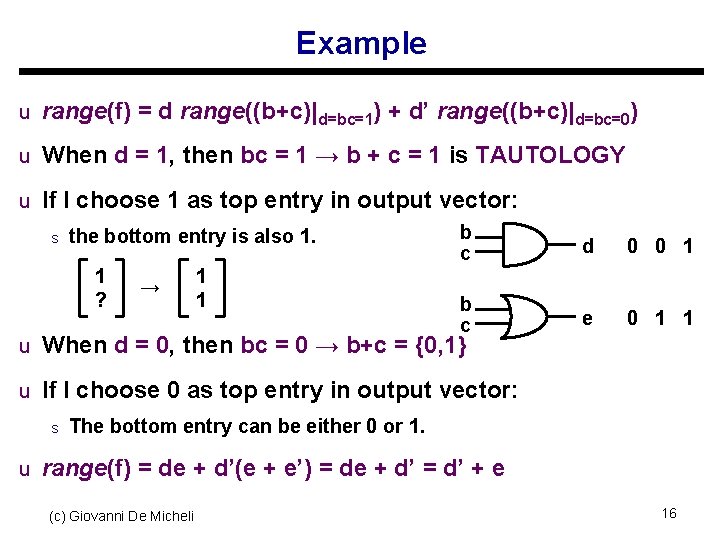
Example u range(f) = d range((b+c)|d=bc=1) + d’ range((b+c)|d=bc=0) u When d = 1, then bc = 1 → b + c = 1 is TAUTOLOGY u If I choose 1 as top entry in output vector: b s the bottom entry is also 1. c 1 1 → ? 1 b c u When d = 0, then bc = 0 → b+c = {0, 1} d 0 0 1 e 0 1 1 u If I choose 0 as top entry in output vector: s The bottom entry can be either 0 or 1. u range(f) = de + d’(e + e’) = de + d’ = d’ + e (c) Giovanni De Micheli 16

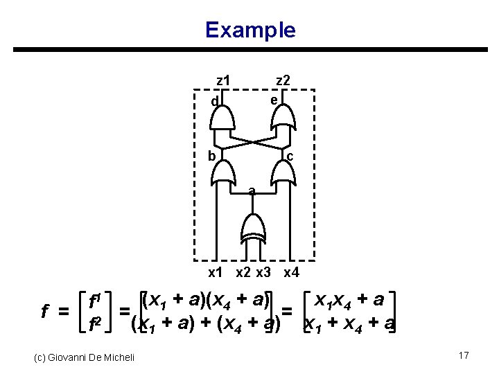
Example z 1 d z 2 e b c a x 1 x 2 x 3 x 4 f = (x 1 + a)(x 4 + a) x 1 x 4 + a f 1 = = 2 (x 1 + a) + (x 4 + a) x 1 + x 4 + a f (c) Giovanni De Micheli 17

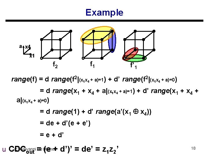
Example a x 4 x 1 f 2 f 1 f’ 1 range(f) = d range(f 2|(x 1 x 4 + a)=1) + d’ range(f 2|(x 1 x 4 + a)=0) = d range(x 1 + x 4 + a|(x 1 x 4 + a)=1) + d’ range(x 1 + x 4 + a|(x 1 x 4 + a)=0) = d range(1) + d’ range(a’(x 1 x 4)) = de + d’(e + e’) = e + d’ (c) Giovanni = De Micheli u CDC (e + d’)’ = de’ = z 1 z 2’ out 18

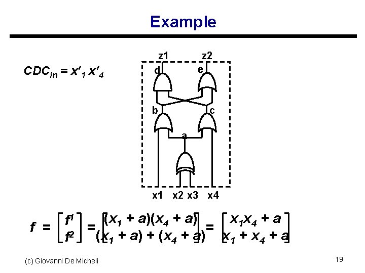
Example CDCin = x’ 1 x’ 4 z 1 d z 2 e b c a x 1 x 2 x 3 x 4 f = (x 1 + a)(x 4 + a) x 1 x 4 + a f 1 = = 2 (x 1 + a) + (x 4 + a) x 1 + x 4 + a f (c) Giovanni De Micheli 19

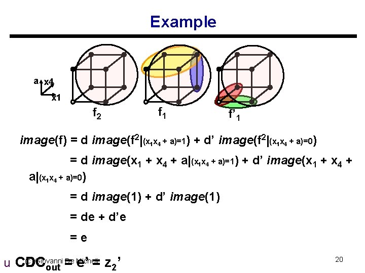
Example a x 4 x 1 f 2 f 1 f’ 1 image(f) = d image(f 2|(x 1 x 4 + a)=1) + d’ image(f 2|(x 1 x 4 + a)=0) = d image(x 1 + x 4 + a|(x 1 x 4 + a)=1) + d’ image(x 1 + x 4 + a|(x 1 x 4 + a)=0) = d image(1) + d’ image(1) = de + d’e =e (c) Giovanni = De Micheli u CDC e’ = z 2’ out 20

Observability analysis u Complementary to controllability s Analyze network from outputs to inputs u More complex because network has several outputs and observability depends on output u Observability may be understood in terms of perturbations s If you flip the polarity of a signal at net x, and there is no change in the outputs, then x is not observable (c) Giovanni De Micheli 21

Observability don’t care conditions u Conditions under which a change in polarity of a signal x is not perceived at the output u If there is an explicit representation of the function, the ODC is the complement of the Boolean difference ODC = ( ∂f / ∂x)’ u Often, the terminal behavior is described implicitly Applying chain rule to Boolean difference is computationally hard (c) Giovanni De Micheli s 22

Tree-network traversal u Consider network from outputs to input u At root s ODCout is given s It may be empty u At internal nodes: s Local function y = fy(x) s ODCx = (∂fy / ∂x )’ + ODCy u Observability don’t care set has two components: Observability of the local function and observability of 23 (c) Giovanni De Micheli the network beyond the local block s

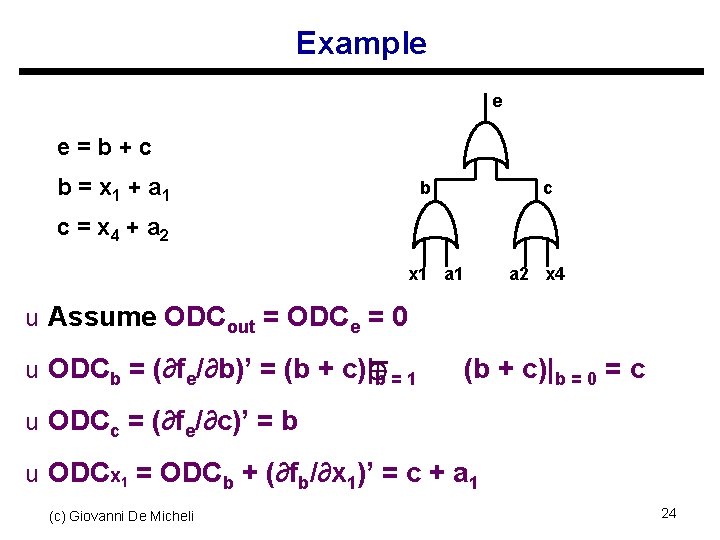
Example e e=b+c b = x 1 + a 1 b c c = x 4 + a 2 x 1 a 2 x 4 u Assume ODCout = ODCe = 0 u ODCb = (∂fe/∂b)’ = (b + c)| b = 1 (b + c)|b = 0 = c u ODCc = (∂fe/∂c)’ = b u ODCx 1 = ODCb + (∂fb/∂x 1)’ = c + a 1 (c) Giovanni De Micheli 24

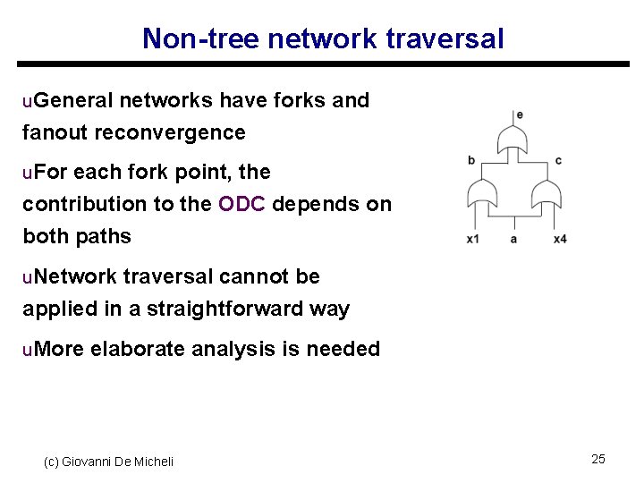
Non-tree network traversal u. General networks have forks and fanout reconvergence u. For each fork point, the contribution to the ODC depends on both paths u. Network traversal cannot be applied in a straightforward way u. More elaborate analysis is needed (c) Giovanni De Micheli 25

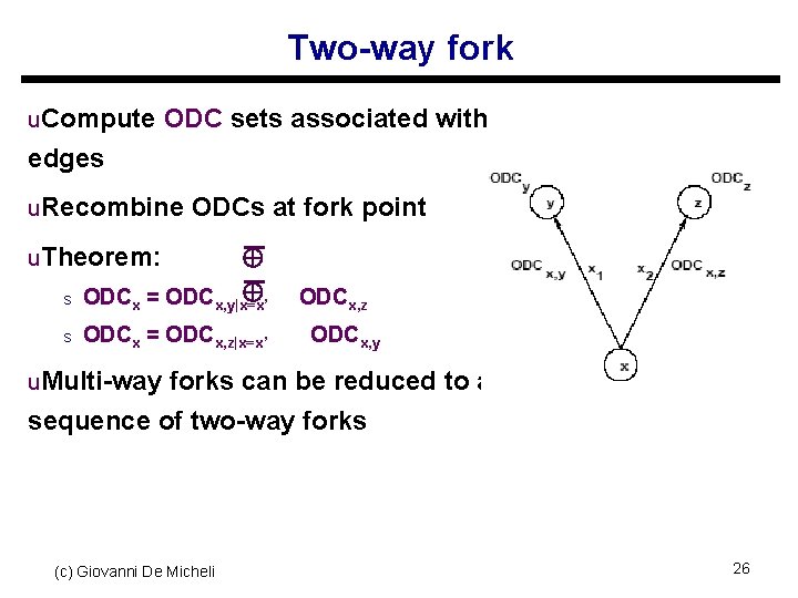
Two-way fork u. Compute ODC sets associated with edges u. Recombine ODCs at fork point s ODCx = ODCx, y|x=x’ s ODCx = ODCx, z|x=x’ u. Theorem: ODCx, z ODCx, y u. Multi-way forks can be reduced to a sequence of two-way forks (c) Giovanni De Micheli 26

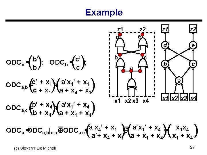
Example z 1 d z 2 e z 1 z 2 d e () () ODC ( =c’ + x )=( a’x ’ + x ) c+x a+x +x ODC ( =b’ + x )=( a’x ’ + x ) b+x a+x +x ODC =ODC | ODC =(a x ’ + x ) ( a’x ’ + x )=( x x ) a’+ x a + x x +x b ODCc = b’ ; ODCb = c’ ; b c a, b 1 4 1 c b a a 1 4 1 x 2 x 3 x 4 x 1 x 2 x 3 x 4 a, c a 4 4 a, b a=a’ 1 4 a, c 4 1 4 (c) Giovanni De Micheli c 1 1 4 1 4 27

Don’t care computation summary u Controllability don’t cares are derived by image computation s Recursive algorithms and data structure applied u Observability don’t cares are derived by backward traversal s Exact and approximate computation s Approximate methods compute don’t care subsets (c) Giovanni De Micheli 28

Transformations with don’t cares u Boolean simplification s Generate local DC set for local functions s Use heuristic minimizer (e. g. , Espresso) s Minimize the number of literals u Boolean substitution: s Simplify a function by adding one (ore more) inputs s Equivalent to simplification with global don’t care sets (c) Giovanni De Micheli 29

Example – Boolean substitution u Substitute q = a + cd into fh = a + bcd + e s Obtain fh = a + bq + e u Method s Compute SDC including q (a+cd) = q’a +q’cd + qa’(cd)’ s Simplify fh = a + bcd + e with DC = q’a + q’cd + qa’ (cd)’ s Obtain fh = a + bq +e u Result s Simplified function has one fewer literal by changing the support of fh (c) Giovanni De Micheli 30

Simplification operator u Cycle over the network blocks s Compute local don’t care conditions s Minimize u Issues: s Don’t care sets change as blocks are being simplified s Iteration may not have a fixed point s It would be efficient to parallelize some simplifications (c) Giovanni De Micheli 31

Optimization and perturbation u Minimizing a function at a block x is the replacement of a local function fx with a new function gx u This is equivalent to perturbing the network locally by s δx = f x g x u Conditions for a feasible replacement s s Perturbation bounded by local don’t care sets δx included in DCext + ODC + CDC (c) Giovanni De Micheli u Smaller, approximate don’t care sets can be 32

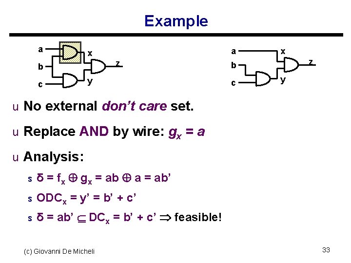
Example a z b c a x y x z b c y u No external don’t care set. u Replace AND by wire: gx = a u Analysis: s δ = fx gx = ab a = ab’ s ODCx = y’ = b’ + c’ s δ = ab’ DCx = b’ + c’ feasible! (c) Giovanni De Micheli 33

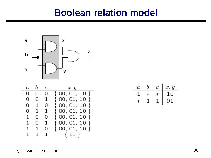
Parallel simplification u Parallel minimization of logic blocks is always possible when blocks are logically independent s Partitioned network u Within a connected network, logic blocks affect each other u Doing parallel minimization is like introducing multiple perturbations s But it is attractive for efficiency reasons u Perturbation analysis shows that degrees of freedom cannot be represented by just an upper bound on the perturbation s Boolean relation model (c) Giovanni De Micheli 34

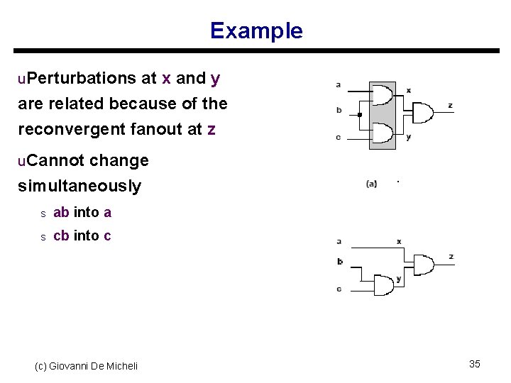
Example u. Perturbations at x and y are related because of the reconvergent fanout at z u. Cannot change simultaneously s ab into a s cb into c (c) Giovanni De Micheli 35

Boolean relation model (c) Giovanni De Micheli 36

Boolean relation model u Boolean relation minimization is the correct approach to handle Boolean optimization at multiple vertices u Necessary steps s Derive equivalence classes for Boolean relation s Use relation minimizer u Practical considerations s High computational requirement to use Boolean relations s Use approximations instead (c) Giovanni De Micheli 37

Parallel Boolean optimization compatible don’t care sets u Determine a subset of don’t care sets which is safe to use in a parallel minimization s Remove those degrees of freedom that can lead to transformations incompatible with others effected in parallel u Using compatible don’t care sets, only upper bounds on the perturbation need to be satisfied u Faster and efficient method (c) Giovanni De Micheli 38

Example u Parallel optimization at two vertices u First vertex x s CODC equal to ODC set s CODCx = ODCx u Second vertex y s CODC is smaller than its ODC to be safe enough to allow for transformations permitted by the first ODC s CODCy = Cx (ODCy) + ODCy ODC’x u Order dependence (c) Giovanni De Micheli 39

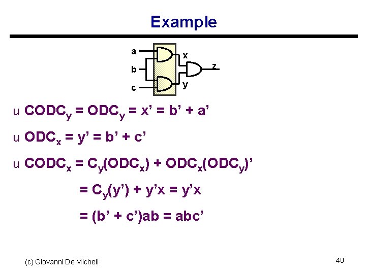
Example a x z b c y u CODCy = x’ = b’ + a’ u ODCx = y’ = b’ + c’ u CODCx = Cy(ODCx) + ODCx(ODCy)’ = Cy(y’) + y’x = (b’ + c’)ab = abc’ (c) Giovanni De Micheli 40

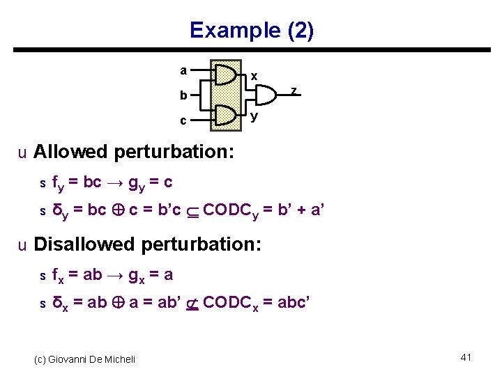
Example (2) a x z b c y u Allowed perturbation: s fy s = bc → gy = c δy = bc c = b’c CODCy = b’ + a’ u Disallowed perturbation: s fx s = ab → gx = a δx = ab a = ab’ CODCx = abc’ (c) Giovanni De Micheli 41

Boolean methods Summary u Boolean methods are powerful means to restructure networks s Computationally intensive u Boolean methods rely heavily on don’t care computation s Efficient methods s Possibility to subset the don’t care sets u Boolean method often change the network substantially, and it is hard to undo Boolean transformations 42 (c) Giovanni De Micheli

Module 2 u Objectives s Testability s Relations between testability and Boolean methods (c) Giovanni De Micheli 43

Testability u Generic term to mean easing the testing of a circuit u Testability in logic synthesis context s Assume combinational circuit s Assume single/multiple stuck-at fault u Testability is referred to as the possibility of generating test sets for all faults s Property of the circuit s Related to fault coverage (c) Giovanni De Micheli 44

Test for stuck-ats u Net y stuck-at 0 s Input pattern that sets y to TRUE s Observe output s Output of faulty circuit differs from correct circuit u Net y stuck-at 1 s Input pattern that sets y to FALSE s Observe output s Output of faulty circuit differs from correct circuit u Testing is based on controllability and observability (c) Giovanni De Micheli 45

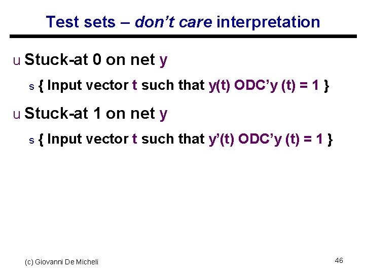
Test sets – don’t care interpretation u Stuck-at 0 on net y s { Input vector t such that y(t) ODC’y (t) = 1 } u Stuck-at 1 on net y s { Input vector t such that y’(t) ODC’y (t) = 1 } (c) Giovanni De Micheli 46

Using testing methods for synthesis u Redundancy removal s Use ATPG to search for untestable fault u If stuck-at 0 on net y is untestable: s Set y = 0 s Propagate constant u If stuck-at 1 on net y is untestable s Set y = 1 s Propagate constant u Iterate for each untestable fault (c) Giovanni De Micheli 47

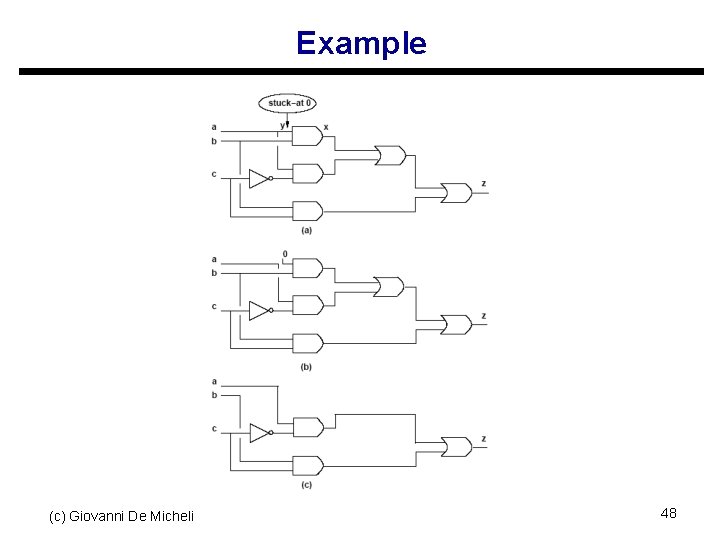
Example (c) Giovanni De Micheli 48

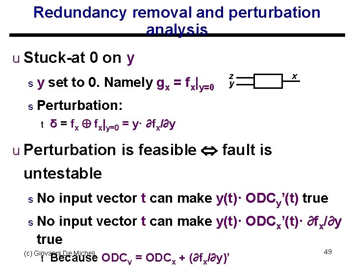
Redundancy removal and perturbation analysis u Stuck-at 0 on y set to 0. Namely gx = fx|y=0 s Perturbation: t z y x δ = fx fx|y=0 = y· ∂fx/∂y u Perturbation is feasible fault is untestable s No input vector t can make y(t)· ODCy’(t) true s No input vector t can make y(t)· ODCx’(t)· ∂fx/∂y true (c) Giovanni De Micheli t Because ODCy = ODCx + (∂fx/∂y)’ 49

Redundancy removal and perturbation analysis u Assume untestable stuck-at 0 fault. u y· ODCx’· ∂fx/∂y SDC u Local don’t care set: s DCx ODCx + y· ODCx’· ∂fx/∂y s DCx ODCx + y· ∂fx/∂y u Perturbation δ = y· ∂fx/∂y s Included in the local don’t care set (c) Giovanni De Micheli 50

Rewiring u Extension to redundancy removal s Add connection in a circuit s Create other redundant connections s Remove redundant connections u Iterate procedure to reduce network s A connection corresponds to a wire s Rewiring modifies gates and wiring structure s Wires may have specific costs due to distance (c) Giovanni De Micheli 51

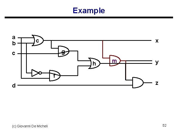
Example a b c x g c h m y f d (c) Giovanni De Micheli z 52

Synthesis for testability u Synthesize fully testable circuits s For single or multiple stuck-at faults u Realizations s Two-level forms s Multi-level networks u Since synthesis can modify the network properties, testability can be addressed during synthesis (c) Giovanni De Micheli 53

Two-level forms u Full testability for single stuck-at faults: s Prime and irredundant covers u Full testability for multiple stuck-at faults s Prime and irredundant cover when t t t Single output function No product-term sharing Each component is prime and irredundant (c) Giovanni De Micheli 54

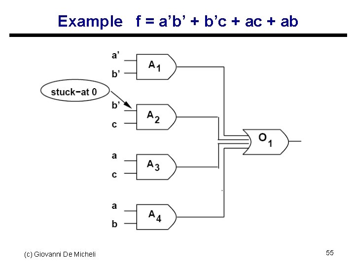
Example f = a’b’ + b’c + ab (c) Giovanni De Micheli 55

Multiple-level networks u Consider logic networks with local functions in sop form u Prime and irredundant network s No literal and no implicant of any local function can be dropped s The AND-OR implementation is fully testable for single stuck-at faults u Simultaneous prime and irredundant network s No subsets of literals and no subsets of implicants can be dropped Giovanni De Micheli s (c)The AND-OR 56 implementation is fully testable for multiple

Synthesis for testability u Heuristic logic minimization (e. g. , Espresso) is sufficient to insure testability of two-level forms u To achieve fully testable networks, simplification has to be applied to all logic blocks with full don’t care sets u In practice, don’t care sets change as neighboring blocks are optimized u Redundancy removal is a practical way of achieving testability properties (c) Giovanni De Micheli 57

Summary – Synthesis for testability u There is synergy between synthesis and testing s Don’t care conditions play a major role in both fields u Testable network correlate to a small area implementation u Testable network do not require to slow-down the circuit u Algebraic transformations preserve multi-fault testability, and are preferable under this aspect (c) Giovanni De Micheli 58