Boolean Logic Networks for Machine Learning Alan Mishchenko

Boolean Logic Networks for Machine Learning Alan Mishchenko University of California, Berkeley (The original work is by Sat Chatterjee from Google AI: “Learning and Memorization”, Proc. ICML’ 18)

Outline l l l Introduction and motivation Proposed architecture Proposed training procedure Experimental results Conclusions and future work 2

Outline l l l Introduction and motivation Proposed architecture Proposed training procedure Experimental results Conclusions and future work 3

Machine Learning (ML) l l l ML learns useful information from application data Data is composed of data samples Data samples are of two types: l l l training set is used for training validation set is used for evaluation of the quality of training ML model is one specific way to do machine learning l neural networks, random forests, etc 4

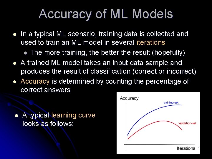
Accuracy of ML Models l l In a typical ML scenario, training data is collected and used to train an ML model in several iterations l The more training, the better the result (hopefully) A trained ML model takes an input data sample and produces the result of classification (correct or incorrect) Accuracy is determined by counting the percentage of correct answers A typical learning curve looks as follows: 5

Motivation l l Neural networks are extensively used As ML models, they have several drawbacks l l l Training takes a lot of time and power Evaluation has high latency (10 K – 1 M cycles) Evaluation is not easy to implement in hardware (resulting in the need for “hardware accelerators”) Design and deployment of hardware accelerators takes a substantial manual effort Can we overcome at least some of these drawbacks by designing a different ML model? 6

Outline l l l Introduction and motivation Proposed architecture Proposed training procedure Experimental results Conclusions and future work 7

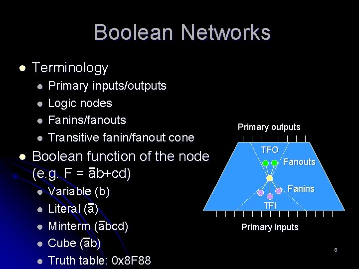
Boolean Networks l Terminology l l l Primary inputs/outputs Logic nodes Fanins/fanouts Transitive fanin/fanout cone Boolean function of the node (e. g. F = ab+cd) l l l Variable (b) Literal (a) Minterm (abcd) Cube (ab) Truth table: 0 x 8 F 88 Primary outputs TFO Fanouts Fanins TFI Primary inputs 8

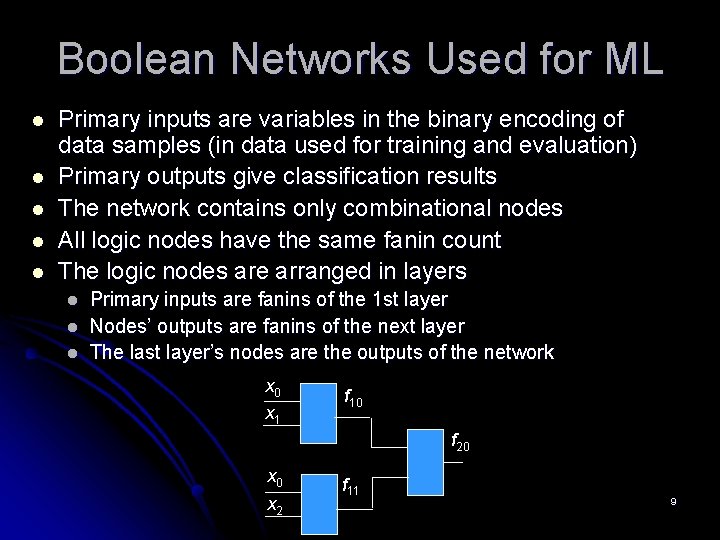
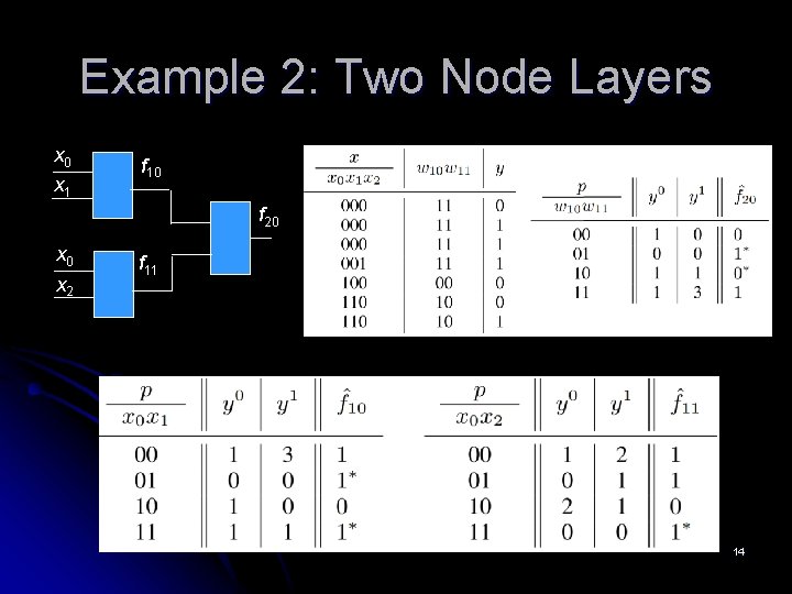
Boolean Networks Used for ML l l l Primary inputs are variables in the binary encoding of data samples (in data used for training and evaluation) Primary outputs give classification results The network contains only combinational nodes All logic nodes have the same fanin count The logic nodes are arranged in layers l l l Primary inputs are fanins of the 1 st layer Nodes’ outputs are fanins of the next layer The last layer’s nodes are the outputs of the network x 0 x 1 f 10 f 20 x 2 f 11 9

Comparison with Neural Networks l Similarities l Computation is arranged in layers l Limited support (of nodes and of CNN neurons) l Similar trends in memorization and generalization (we will see this later) l Differences l Currently, training in one pass, by memorization l without back-propagation l without gradient descent l without any explicit search 10

Outline l l l Introduction and motivation Proposed architecture Proposed training procedure Experimental results Conclusions and future work 11

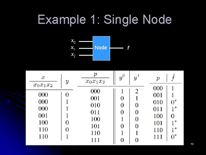
Formal Description l l l Consider the problem of learning a function f : Bk → B from a list of training pairs (x, y) where x Bk and y B To learn by memorizing, first construct a table of 2 k rows (one for each pattern p Bk) and two columns, y 0 and y 1 The y 0 entry for the row p (denoted by cp 0) counts how many times p leads to 0, i. e. , the number of times (p, 0) occurs in the training set Similarly, the y 1 entry for row p (denoted by cp 1) counts how many times p leads to output 1 in the training set Associate function f(p) : Bk → B with the table as follows: 1 if cp 1 > cp 0 f(p) = 0 if cp 1 < cp 0 b if cp 1 = cp 0 12 where b B is picked uniformly at random {

Example 1: Single Node x 0 x 1 x 2 Node f 13

Example 2: Two Node Layers x 0 x 1 f 10 f 20 x 2 f 11 14

Analysis of Training Procedure l The procedure is linear in the size of the training data, with two passes over the data on each layer l l l It is efficient since it involves only counting and node evaluation and does not use floating point l l first, counting input patterns second, comparing counters and assigning the output uses only memory lookups and integer addition It is easily parallelizable l l each node in a layer is independent the occurrence counts can be computed for disjoint subsets of the training data and added together 15

Outline l l l Introduction and motivation Proposed architecture Proposed training procedure Experimental results Conclusions and future work 16

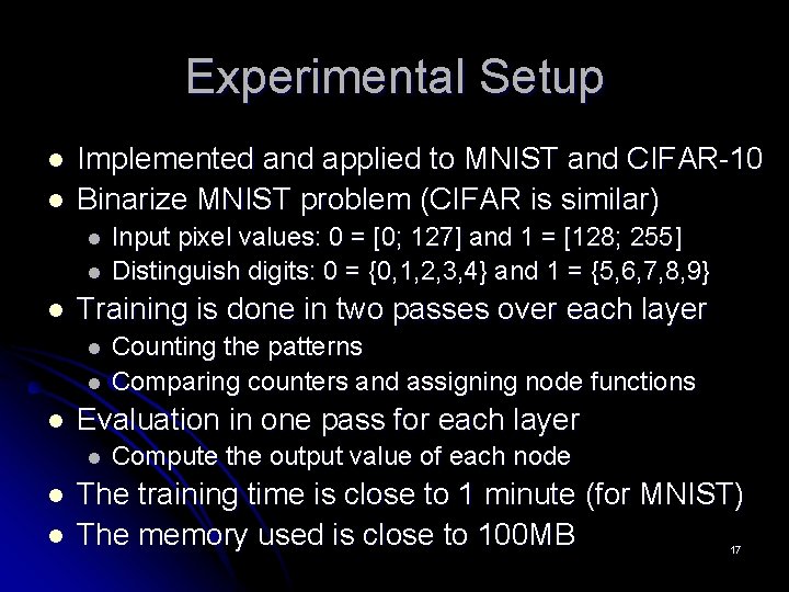
Experimental Setup l l Implemented and applied to MNIST and CIFAR-10 Binarize MNIST problem (CIFAR is similar) l l l Training is done in two passes over each layer l l Counting the patterns Comparing counters and assigning node functions Evaluation in one pass for each layer l l Input pixel values: 0 = [0; 127] and 1 = [128; 255] Distinguish digits: 0 = {0, 1, 2, 3, 4} and 1 = {5, 6, 7, 8, 9} Compute the output value of each node The training time is close to 1 minute (for MNIST) The memory used is close to 100 MB 17

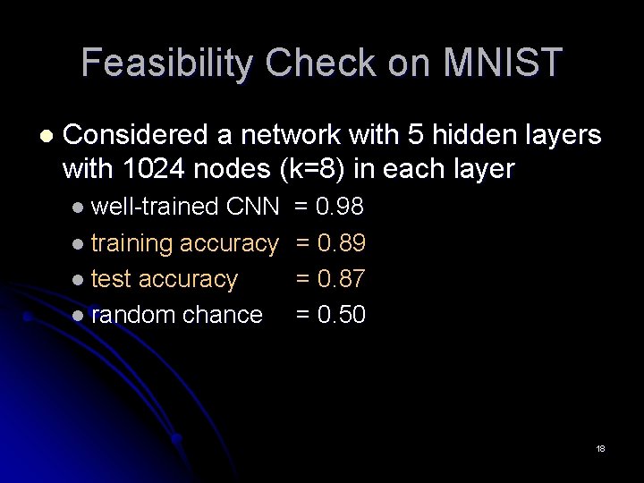
Feasibility Check on MNIST l Considered a network with 5 hidden layers with 1024 nodes (k=8) in each layer l well-trained CNN l training accuracy l test accuracy l random chance = 0. 98 = 0. 89 = 0. 87 = 0. 50 18

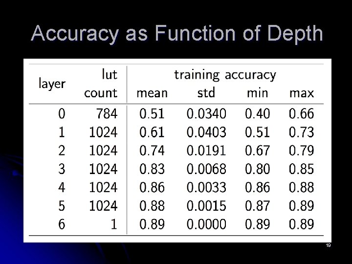
Accuracy as Function of Depth 19

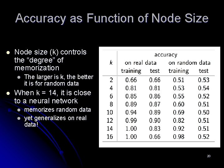
Accuracy as Function of Node Size l Node size (k) controls the “degree” of memorization l l The larger is k, the better it is for random data When k = 14, it is close to a neural network l l memorizes random data yet generalizes on real data! 20

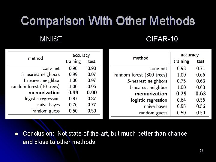
Comparison With Other Methods MNIST l CIFAR-10 Conclusion: Not state-of-the-art, but much better than chance and close to other methods 21

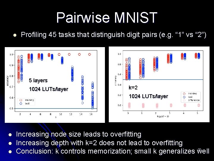
Pairwise MNIST l Profiling 45 tasks that distinguish digit pairs (e. g. “ 1” vs “ 2”) 5 layers 1024 LUTs/layer k=2 1024 LUTs/layer l l l Increasing node size leads to overfitting Increasing depth with k=2 does not lead to overfitting 22 Conclusion: k controls memorization; small k generalizes well

Pairwise CIFAR-10 23

Outline l l l Introduction and motivation Proposed architecture Proposed training procedure Experimental results Conclusion and future work 24

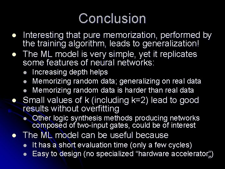
Conclusion l l Interesting that pure memorization, performed by the training algorithm, leads to generalization! The ML model is very simple, yet it replicates some features of neural networks: l l Small values of k (including k=2) lead to good results without overfitting l l Increasing depth helps Memorizing random data; generalizing on real data Memorizing random data is harder than real data Other logic synthesis methods producing networks composed of two-input gates, could be of interest The ML model can be useful because l l It has a short evaluation time (only a few cycles) Easy to design (no specialized “hardware accelerator”) 25

Future Work Is this approach useful in practice? l Can the accuracy be improved? l How to extend beyond binary classification? l Need better theoretical understanding l 26

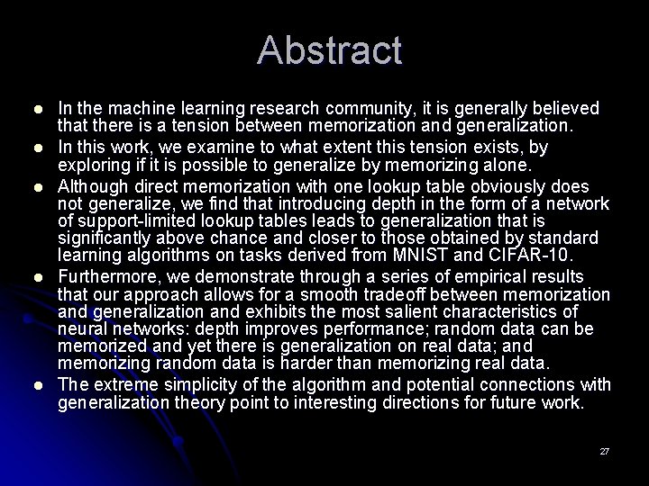
Abstract l l l In the machine learning research community, it is generally believed that there is a tension between memorization and generalization. In this work, we examine to what extent this tension exists, by exploring if it is possible to generalize by memorizing alone. Although direct memorization with one lookup table obviously does not generalize, we find that introducing depth in the form of a network of support-limited lookup tables leads to generalization that is significantly above chance and closer to those obtained by standard learning algorithms on tasks derived from MNIST and CIFAR-10. Furthermore, we demonstrate through a series of empirical results that our approach allows for a smooth tradeoff between memorization and generalization and exhibits the most salient characteristics of neural networks: depth improves performance; random data can be memorized and yet there is generalization on real data; and memorizing random data is harder than memorizing real data. The extreme simplicity of the algorithm and potential connections with generalization theory point to interesting directions for future work. 27