Book 2 name for CIT421 Book name for

Book 2 name for CIT-421

Book name for CIT-421

Image formats

Image data types • Binary images are 2 -D arrays that assign one numerical value from the set {0; 1} to each pixel in the image. These are sometimes referred to as logical images: black corresponds to zero (an ‘off’ or ‘background’ pixel) and white corresponds to one (an ‘on’ or ‘foreground’ pixel). • Intensity or grey-scale images are 2 -D arrays that assign one numerical value to each pixel which is representative of the intensity at this point. • RGB or true-colour images are 3 -D arrays that assign three numerical values to each pixel, each value corresponding to the red, green and blue (RGB) image channel component respectively. • Floating-point images store a floating-point number which, within a given range defined by the floating-point precision of the image bit resolution, represents the intensity. They may (commonly) represent a measurement value other than simple intensity or colour as part of a scientific or medical image.

Thresholding • Thresholding produces a binary image from a grey-scale or colour image by setting pixel values to 1 or 0 depending on whether they are above or below the threshold value. • Thresholding operates on an image I as follows:
 Functional transformation of Image: • The dynamic range of")
Point-based operations on images (p-57) Functional transformation of Image: • The dynamic range of an image is defined as the difference between the smallest and largest pixel values within the image. • Functional transforms or mappings that alter the effective use of the dynamic range. These transforms are primarily applied to improve the contrast of the image. • In general, we will assume an 8 -bit (0 to 255) grey-scale range for both input and resulting output images

Logarithmic transform • The dynamic range of an image can be compressed by replacing each pixel value in a given image with its logarithm: Ioutput(i, j) = ln Iinput (i, j) where I(i, j) is the value of a pixel at a location (i, j) in image I and the function ln() represents the natural logarithm. • In practice, as the logarithm is undefined for zero, the following general form of the logarithmic transform is used: • Note that the scaling factor controls the input range to the logarithmic function, whilst c scales the output over the image quantization range 0 to 255. • The addition of 1 is included to prevent problems where the logarithm is undefined for Iinput(i, j) = 0.

• The level of dynamic range compression is effectively controlled by the parameter • Figure 3. 6 The Logarithmic Transform: Varying the parameter changes the gradient of the logarithmic function used for input to output

• To increase the dynamic range of dark regions in an image and decrease the dynamic range in the light regions. • Thus, the logarithmic transform maps the lower intensity values or dark regions into a larger number of grey scale values and compresses the higher intensity values or light regions in to a smaller range of grey scale values. • Figure 3. 7 Applying the logarithmic transform to a sample image

• By applying the logarithmic transform we brighten the foreground of this image by spreading the pixel values over a wider range and revealing more of its detail whilst compressing the background pixel range. • The scaling constant c can be calculated based on the maximum allowed output value (255 for an 8 -bit image) and the maximum value max (Iinput (i, j)) present in the input:

Exponential transform • The exponential transform is the inverse of the logarithmic transform. Here, the mapping function is defined by the given base e raised to the power of the input pixel value: • where I(i, j) is the value of a pixel at a location (i, j) in image I. • This transform enhances detail in high-value regions of the image (bright) whilst decreasing the dynamic range in low-value regions (dark) – the opposite effect to the logarithmic transform. • In general, base numbers just above 1 are suitable for photographic image enhancement. Thus, we expand our exponential transform notation to include a variable base and scale to the appropriate output range as before:

• Here, is the base and c is the scaling factor, the exponential function is close to linear the origin, the compression is greater for an image containing a lower range of pixel values than one containing a broader range. • Figure 3. 8 The Exponential Transform: Varying the parameter changes the gradient of the exponential function used for input to output

• The contrast of the background in the original image can be improved by applying the exponential transform, but at the expense of contrast in the darker areas of the image. • The background is a high-valued area of the image (bright), whilst the darker regions have low pixel values. This effect increases as the base number is increased. • Figure 3. 9 Applying the exponential transform to a sample image

Pixel distributions: histograms • An image histogram is a plot of the relative frequency of occurrence of each of the permitted pixel values in the image against the values themselves. • If we normalize such a frequency plot, so that the total sum of all frequency entries over the permissible range is one, we may treat the image histogram as a discrete probability density function which defines the likelihood of a given pixel value occurring within the image. • Visual inspection of an image histogram can reveal the basic contrast that is present in the image and any potential differences in the colour distribution of the image foreground and background scene components. • For a simple grey-scale image, the histogram can be constructed by simply counting the number of times each grey-scale value (0– 255) occurs within the image. • Each ‘bin’ within the histogram is incremented each time its value is encountered

• Histogram plot with two distinctive peaks: a high peak in the lower range of pixel values corresponds to the background intensity distribution of the image and a lower peak in the higher range of pixel values (bright pixels) corresponds to the foreground objects (coins). • Figure 3. 12 Sample image and corresponding image histogram
 • If")
When is it necessary to modify the histogram of an image? (p-367) • If we cannot see much detail in an image, the reason could be that pixels, which represent different objects or parts of objects, have grey values which are very similar to each other. • The histogram of the “bad” image is very narrow and it does not occupy the full range of possible grey values, while the histogram of the “good” image is more spread.

Histograms for threshold selection • By selecting a threshold value between the two histogram peaks we can successfully separate the background/foreground of the image using the thresholding approach. • For calculation of an automatic threshold value the Otsu method, which chooses that threshold value which minimizes the interclass statistical variance of the thresholded black and white pixels, is used. • In Figure 3. 12, the x-axis represents the range of values within the image (0– 255 for 8 -bit grayscale) and the y-axis shows the number of times each value actually occurs within the particular image. • The threshold of 120 is suitable for Figure 3. 12.

• For more complex scenes, such as Figure 3. 13, a more complex histogram occurs and simple foreground/background thresholding cannot be applied. • In suchcases, we must resort to more sophisticated image segmentation techniques.

Adaptive thresholding • Adaptive thresholding is designed to overcome the limitations of conventional, global thresholding by using a different threshold at each pixel location in the image. This local threshold is generally determined by the values of the pixels in the neighbourhood of the pixel. • Adaptive thresholding works from the assumption that illuminationmay differ over the image but can be assumed to be roughly uniformin a sufficiently small, local neighbourhood. • The local threshold value t in adaptive thresholding can be based on several statistics. • Typically, the threshold is chosen to be either t = mean + C , t = median + C, or floor((max-min)/2) + C of the local N × N pixel neighbourhood surrounding each pixel.

• The threshold t = mean + C for a neighbourhood of N = 15 and C = 20. The result of this example is shown in Figure 3. 14, where we see the almost perfect foreground separation of the rice grains. • Figure 3. 14 Adaptive thresholding applied to sample image

Contrast stretching • Image histograms are also used for contrast stretching (also known as normalization) which operates by stretching the range of pixel intensities of the input image to occupy a larger dynamic range in the output image. • The upper and lower limits of the pixel quantization range in use (i. e. for an 8 -bit image, a = 255 and b = 0. • The maximum and minimum pixel values currently present, denoted c and d respectively. • The image pixel range is stretched according to the following formula: • for each pixel location denoted I(i, j) in the input and output images.

Two such methods, for selecting c and d, are presented here. • Method 1: Compute the histogram of the input image and select c and d as the 5 th and 95 th percentile points of the cumulative distribution (i. e. 5% of the image pixels will be less than c and 5% greater than d). • Method 2: Compute the histogram of the input image and find the most frequently occurring intensity value within the image. • Let us assume that this peak value has a bin count of N. Select as a cut-off some fraction of N (e. g. 5%). Move away from the peak in either direction (left towards 0 one way, right towards 255) until the last values greater than the cut-off are reached. These values are c and d (see the histogram in Figure 3. 12).

Contrast stretching by using method 1 to image and histogram distribution

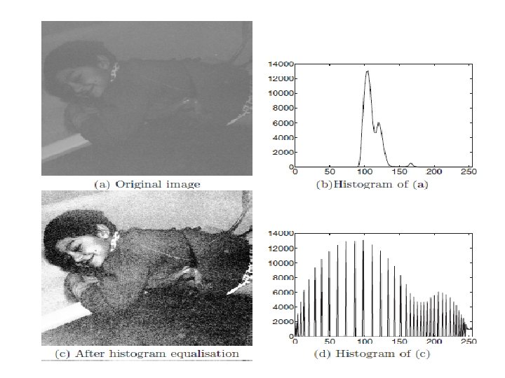
Histogram equalization • The second contrast enhancement operation based on the manipulation of the image histogram is histogram equalization. This is one of the most commonly used image enhancement techniques. Histogram equalization in practice • In histogram equalization, we employ a monotonic, nonlinear mapping such that the pixels of the input image are mapped to an output image with a uniform histogram distribution. • In the idealized case, the resulting equalized image will contain an equal number of pixels each having the same grey level. • For L possible grey levels within an image that has N pixels, this equates to the jth entry of the cumulative histogram C(j) having the value j. N/L in this idealized case (i. e. j times the equalized value).

We can thus find a mapping between input pixel intensity values i and output pixel intensity values j as follows: (3. 17) from which rearrangement gives: (3. 18) • which represents a mapping from a pixel of intensity value i in the input image to an intensity value of j in the output image via the cumulative histogram C() of the input image.

• Notably, the maximum value of j from the above is L, but the range of grey-scale values is strictly j = {0…(L-1)} for a given image. In practice this is rectified by adding a-1 to the equation, thus also requiring a check to ensure a value of j =-1 is not returned: (3. 19) • which, in terms of our familiar image-based notation, for 2 -D pixel locations i = (c, r) and j = (c, r) transforms to (3. 20) • where C() is the cumulative histogram for the input image Iinput, N is the number of pixels in the input image (C×R) and L is the number of possible grey levels for the images.
- Slides: 28