Bondi 1952 Bondi H On spherically symmetrical accretion

Bondi, 1952 (Bondi, H. , On spherically symmetrical accretion, Monthly Notices of the Royal Astronomical Society, Vol. 112, № 2, p. 195 -204, 1952)

Map of the Local Bubble in the Galactic plane, where the contours indicate 20 mÅ and 50 mÅ equivalent widths for the Na I D 2 line (Lallement et al. , 2003). The distance scale is in parsecs.

HST/GHRS spectra of the Ly lines of Cen A and B, showing broad absorption from interstellar H I and narrow absorption from D I (Linsky and Wood, 1996).

Schematic diagram showing how a stellar Ly profile changes from its initial appearance at the star and then through various regions that absorb parts of the profile before it reaches an observer at Earth: the stellar astrosphere, the LISM, and finally the heliosphere (Wood et al. , 2003 b). The lower panel shows the actual observed Ly profile of Cen B. The upper solid line is the assumed stellar emission profile and the dashed line is the ISM absorption alone. The excess absorption is due to heliospheric H I (green shading) and astrospheric H I (red shading).
 • Turbulent and laminar transports of energy, momentum and mass in")
Short resume (1) • Turbulent and laminar transports of energy, momentum and mass in the hot solar corona and at the cooler transition region/ chromospheric levels of the solar atmosphere finally result in the permanent, but strongly variable supermagnetosonic plasma outflow from the Sun: the solar wind. This view differs from past laminar theories of the coronal heating and the solar wind formation.
 • Many important aspects of this general astrophysical and plasma physical")
Short resume (2) • Many important aspects of this general astrophysical and plasma physical phenomenon are known due to numerous spacecraft measurements, as well as various remote sensing methods. In spite of rapidly increasing information and knowledge, there is no sufficiently deep physical understanding of the connection between observed phenomena, structures and parameters on the Sun and measured properties of the solar wind in the heliosphere.
 • In the present review, we will cross this bridge between")
Short resume (3) • In the present review, we will cross this bridge between the Sun and the heliosphere in both directions, attentively looking at known and clear manifestations, observations and models which are well investigated. We will mark unclear and questionable details, as well as the points of obvious disagreement with the current wisdom. The last is probably most important for the further steps in theory and observations.

Methods • We will analyze available data sets about laminar and turbulent regimes (weak, moderate and strong ones including discontinuities and shocks) and combine them with theories, analytical and numerical models in attempts to summarize and develop modern understanding of longstanding problems related to the solar wind origins. • The work is supported by the INTAS grant 03 -51 -6206, the Russian Foundation for Basic Research grants 07 -0207012, 06 -05 -64500, and contributes to the Projects of the Russian Academy of Sciences Programs P 04, P 30, OFN 16 and the Interdisciplinary MSU Program.

Three important aspects • There are three important aspects of the solar wind origins problem that we are aimed to focus on: • 1) overall and global solar wind flow as a stellar phenomenon; • 2) large-scale and long-term quasi-stationary structure; • 3) small-scale and transient self-organization. • All three aspects are mutually related by complicated non-linear couplings, which are not well investigated and described.

Solar wind as a result of the stellar evolution • The Solar System and the Sun formation processes, according to modern cosmogenic hypotheses, started as an accretion from the local interstellar gas-dust medium mediated by electromagnetic fields and radiation. • Open questions: when and how the accretion was stopped and replaced by the plasma outflow from the Sun?
 plotted versus X-ray surface flux (Wood")
Measured mass loss rates (per unit surface area) plotted versus X-ray surface flux (Wood et al. , 2005 a). The filled and open circles are main sequence and evolved stars, respectively. For the main sequence stars with , mass loss appears to increase with coronal activity, so a power law has been fitted to these stars, and the shaded region is the estimated uncertainty in the fit. The saturation line represents the maximum

Bondi’s model consideration • • The model of the steady state spherically symmetric flows of the politrope gas in the gravity field of the central star body was first developed by Bondi (1952). He obtained and investigated the whole family of subsonic, transsonic and supersonic solutions of the reduced Bernoulli equation. The same family of Bernoulli equation solutions was used for the description of possible inflows to the Sun - accretion (Bondi, 1952) and outflows - solar wind (Parker, 1958). Dilemma. The selection between positive or negative branches for the radial velocity can be not uniquely decided in the framework of this steady state approach without additional hypotheses about external boundary conditions in the interstellar medium and internal conditions on the Sun. Physical analogy: electrons and positrons in the field theory. Mixed and intermittent accretion and wind regimes are easily reproduced by the same Bondi model. Transitions between those regimes are not excluded and possible.

Entropy considerations • Not helpful to resolve the ‘accretion-wind’ dilemma. • It is because of physically open system including given star and its surroundings should be considered. • Entropy increases in closed physical systems, but it could locally decrease.

Evolution considerations • Evolving interstellar medium with stars. • Physically open system with energy, momentum and mass flows. • Prehistory and memory of past development bring initial conditions, which are not known a priori from direct observations and could be only speculated. • Time dependence and ‘world line’ can be followed and constructed for future development only within some accuracy. Predictability horizon exists, but not known. • Memory is partially lost due to dissipation. Sufficiently deep past history is not reproducible in principle because of lost information via radiation and mass losses from the finite volume under consideration.

General comments • Only finite volumes and limited time intervals are tractable in physics. • ‘Universe as a whole’ is not a subject for physical considerations because it is not based on necessary and sufficient input information from observations. • Knowledge is limited and will remain limited, though increasing.

Preliminary conclusions from general and evolutionary considerations in application to the solar wind origin problem • Attempts to solve the solar wind problem as the unique situation for stars with a hot corona in a tenuous interstellar medium are physically not tenable. • Two possible branches – wind accretion are admissible for the stars of the solar type. • The selection between two branches is due to evolutionary path, but not to the structure of the stellar interiors. • The dilemma wind/accretion de facto has one and only one evolutionary solution.

Stars as donors and acceptors of the interstellar gas • The current situation in the star - interstellar gas interaction depends on many parameters of a star under consideration and surrounding medium including neighbour stars. • If the evolutionary paths are different, stars can serve as donors or acceptors. • Local solution is impossible for dilemma ‘wind/accretion’.

Comment on the history of science about the solar wind • Correct orders of magnitude for density, velocity and temperature of the solar wind were know from observations long before the Space Era (see e. g. Kiepenheuer, 1953). • The opposite statement by Parker (2007) that “none of pre-Space Age density estimates inferred from observations was correct” (pp. 110 -111 ibid) is in error. • Correct estimates were not appreciated by ‘majority and authority’ in scientific establishment at that time, but it is another story, which has little common with real knowledge. • The history continues… • • Kiepenheuer K. O. (1953). Solar Activity, “The Sun” Edited by Gerard P. Kuiper. Chicago: The University of Chicago Press, 1953, p. 322 Parker E. N. (2007). Solar wind, in Y. Kamide and A. Chian (Eds. ), “Handbook of the Solar-Terrestrial Environment”, Springer, Berlin, 2007.

Contents • Dimensionless parameters in MHD with dissipation and radiation • Eruptions with/without topological changes (‘reconnection’) • Velocity scaling and velocity ‘reconnection’ • Classical case interpretation (eruption of May 15, 1919 on the Sun) • Conclusions

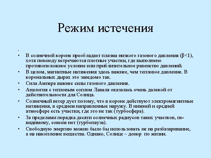
Turbosphere around the Sun • Up-and -down flows. Lateral motions of plasma. • Transient (S<<1) and quasi steady (S>>1) regimes. • Subsonic M<<1, trans-sonic M~1 and super magnetosonic M>>1 cases. M here stays for MS, , MA or their combinations (slow and fast magnetosonic speeds). • Spicules, macrospicules, jets, eruptions demonstrate confined (finite) and infinite trajectories of moving particles in the chromosphere and the corona. • Solar wind originates as a tiny regular outflow superimposed on the background of more powerful irregular (turbulent) motions. Some of these motions are inbound and returning to the Sun, but outbound motions dominate more and more with distance from the surface. • Illustrations are on the next slides.

Turbopause around the Sun • Definition. • Turbopause is the instant surface where the local turbulent velocity (Vturb) is approximately equal to the average and regular speed of the radial plasma outflow V. • Below the turbopause: Vturb > V. • Above the turbopause: V > Vturb.
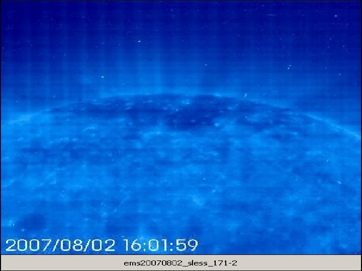
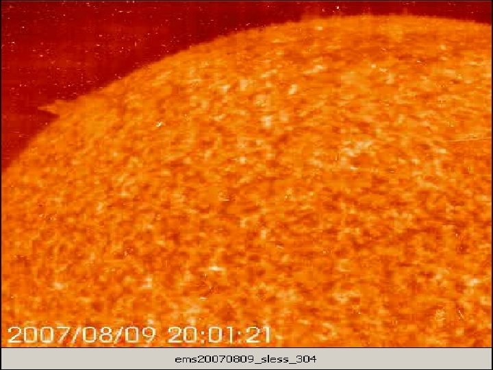
 onboard SOHO •")
Shuttrless • High-cadence synoptic program of the Extremeultraviolet Imaging Telescope (''Shutterless'') onboard SOHO • Frederic Clette et al. (http: //sidc. be/EIT/High-cadence/). • (Active Regions, Quiet Sun, Coronal Holes, etc. ). • Wide field of view (~ a quarter of the disc). • 68 s cadence with an effective exposure larger than the standard synoptic exposures (best for CH and QS). • Transition Region as well as the corona: sequences alternately in 2 bandpasses: 304Å and 195Å (with occasionally a third one: 171Å).
 magnetic field B; 2) mass density ρ")
Dimensionless scaling: Alfvén wave • Given: 1) magnetic field B; 2) mass density ρ • Problem: Find characteristic velocity of perturbations • Answer: (H. Alfvén, 1942) VA ~ B/ρ1/2
 • Given: 1) Strong point-like")
Dimensionless scaling: strong explosions in the atmosphere (Sedov’s solution) • Given: 1) Strong point-like explosion in the homogeneous atmosphere 2) E - energy released 3) ρ -density of the atmosphere 4) t – time after explosion • Problem: Find the shock velocity u(t) as a function of time • Solution: Dimensionless parameter was found ( L. I. Sedov) ξ = r (ρ/E t 2)1/5 • Answer: u(t) ~ (E/ρt 3)1/5 • Practical implications: Energy of the explosion E can be estimated from kinematics of the strong shocks
")
Explosive wave Hinode observations December 6, 2006 (656. 28 nm)

Complicated dynamical geometry of arcades: • Spurious “reconnections” and X-points: projections of twisted loops • Spurious “crossings of the loops”: the same as above • Spurious “plasmoids”: brighter summits of the loops (an example from the TRACE “gold mine”)

Projection effects

Multi-scale nature of erupting prominences

Conservation Laws mass momentum energy

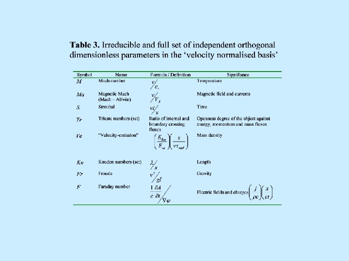
Dimensionless parameters

New interpretation of the classical observation E. Pettit, The Great Eruptive Prominences of May 29 and July 15, 1919, Astrophys. J. , vol. 50, pp. 206 -219, 1919 Internal and External Motions Velocity reconnection Loops and whips E. Pettit does not addmitted external motions

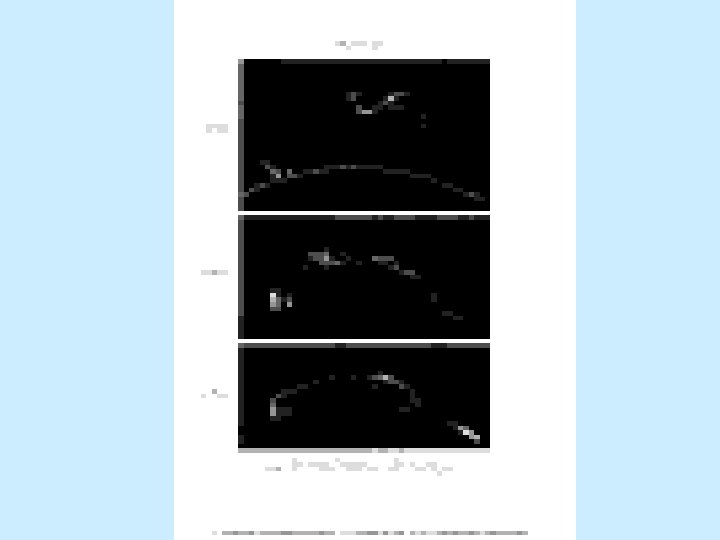
May 15, 1919 huge prominence on the East limb 8 hours rise up to 2 solar radii stereo couples and velocity tracing a loop transformed into a whip

Height versus time
")
Detailed stereoscopic velocity measurements (0 - ~ 100 km/s)

Simple velocity model siphon flow+solar wind= whip formation

Strouhal number • S ~ vt/L non-invariant, reference frame dependent parameter • S>>1 quasi-stationary flow (asymptotically large S values mean steady state) • S<<1 transient flow • S~1 intermediate regime (for example, linear waves or small convective perturbations)
 • S ~ Vt/L • Quiescent prominences: • L~ 105 km,")
Strouhal number (ctnd) • S ~ Vt/L • Quiescent prominences: • L~ 105 km, V~ 1 km/s, t~ 106 s (many days, a month) (life time) • Hence, S ~ 10 • Looks like quasi-steady flows during life time
 • • S ~ vt/L Eruptive prominences: for example, L~ 105")
Strouhal number (ctnd) • • S ~ vt/L Eruptive prominences: for example, L~ 105 km, V~ 100 km/s, t ~ 1 hour Looks like transient phenomenon

Laminar? Turbulent? • Number of degrees of freedom N involved in process under consideration • Laminar if N~ 1 “simple” • Turbulent if N>>1 “complicated” • Reynolds number Re is not invariant for this purpose (reference frame dependent impressions of flow). Because of this, • Re >1, Re <1 is not a good classification.

Dimensionless Faraday number F • Ratio of inductive and potential electric fields • F~ (j/ρc) (L/ct) where j - electric current density ρ - electric charge density L - length c - velocity of light t - time F>>1 inductive fields dominate F<<1 Coulomb fields dominate → electrostatics important! Applications: thermonuclear fusion problem, double layers on the Sun

Trieste numbers T • Set of dimensionless parameters: ratios of energy, momentum , mass fluxes inside, outside and across the volume boundaries • T>>1 open system • T<<1 closed system • T~1 intermediate case • Important example: quiescent prominence – open system with mass flows through it (siphon flows in loops from one foot point to opposite foot point, blue and red shifts in legs). It is not a magneto-static equilibrium (as generally believed) but a quasi-steady or non-steady state with flows

Why solar flares and CMEs originate? • It is because of subphotospheric free energy supply in the same, larger and smaller space-time scales: T~1, T>>1, T<<1. • All these regimes involved in preparation and development • They are non-linearly coupled • Information and ‘signals’ from interior of the Sun are needed to predict solar flares and CMEs
 • Ratio of the energy losses via solar wind")
Ve number (on the Sun) • Ratio of the energy losses via solar wind to the losses due to electromagnetic radiation of the corona • Averages on time : • Ve>>1 in coronal holes (dark regions, fast wind) • Ve<<1 in active regions (bright loops, slow motions) • Ve~1 intermediate value in quiet corona
 • Ve>>1 in coronal mass ejections (CMEs) – high loop eruptions,")
Ve number (continued) • Ve>>1 in coronal mass ejections (CMEs) – high loop eruptions, prominences, arcades • Ve<<1 in solar flares – low loops, brightening, confined motions • Ve~1 intermediate case - both • Typically CMEs and flares are accompanying each other in different proportions from CME-like to flare like situations • Flares/CMEs: No cause/consequence relations, but parallel energy release channels from the same free energy sources

Syrovatsky number • Defined as combination M 2/МA. • Includes temperature, magnetic field, velocity • NOT INCLUDES DENSITY! Comfortable for the classification of incompressible MHD flows • The same M β-1/2 • The same MAβ-1 • Here β ~ (MA/M)2. P/B 2

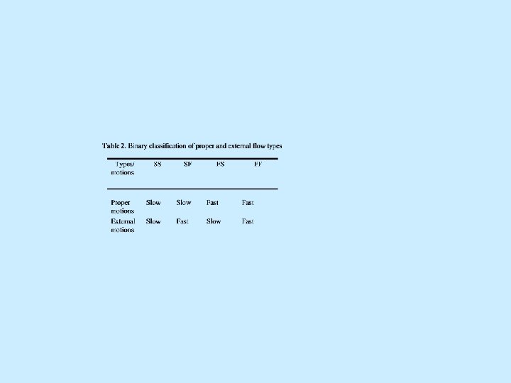
CONCLUSIONS ü Dimensionless velocity scaling gives unambiguous classification of ejection on the Sun. ü 8 binary and 27 ternary types of the velocity field can be indicated. ü Velocity field reconnection is observed during ejection as “loop - whip shape transformation. ” ü Classical observations by E. Pettit are interpreted using this approach: siphon+solar wind= whip. ü Thank you!
- Slides: 65