BOLD f MRI BIAC Graduate f MRI Course

BOLD f. MRI BIAC Graduate f. MRI Course September 28, 2004

Why do we need to know physics/physiology of f. MRI? • To understand the implications of our results – Interpreting activation extent, timing, etc. – Determining the strength of our conclusions – Exploring new and unexpected findings • To understand limitations of our method – Choosing appropriate experimental design – Combining information across techniques to overcome limitations • To take advantage of new developments – Evaluating others’ approaches to problems – Employing new pulse sequences or protocols

Developments for BOLD MRI • Echoplanar imaging methods – Proposed by Mansfield in 1977 • Ready availability of high-field scanners – Technological developments – Clinical applicability insurance reimbursement clinical prevalence • Discovery of BOLD contrast mechanism
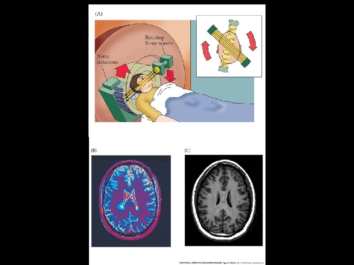

Developments for BOLD MRI • Echoplanar imaging methods – Proposed by Mansfield in 1977 • Ready availability of high-field scanners – Technological developments – Clinical applicability insurance reimbursement clinical prevalence • Discovery of BOLD contrast mechanism

Contrast Agents • Defined: Substances that alter magnetic susceptibility of tissue or blood, leading to changes in MR signal – Affects local magnetic homogeneity: decrease in T 2* • Two types – Exogenous: Externally applied, non-biological compounds (e. g. , Gd-DTPA) – Endogenous: Internally generated biological compound (e. g. , d. Hb)

External Contrast Agents • Most common are Gadolinium-based compounds introduced into bloodstream – Very large magnetic moments – Do not cross blood-brain barrier • Create field gradients within/around vessels – Reduces T 1 values in blood (can help visualize tumor, etc. ) – Changes local magnetic fields • Large signal changes: 30 -50% – Delay until agent bolus passes through MR imaging volume – Width of response depends on delivery of bolus and vascular filtering – Degree of signal change depends on total blood volume of area • Issues – Potential toxicity of agents (short-term toxicity, long-term accumulation) – Cause headaches, nausea, pain at injection
 CBV Maps (+24%)")
Belliveau et al. , 1990 Slice Location NMR intensity change (CBV) CBV Maps (+24%)

Common Contrast Agents Longitudinal Relaxivity Transverse Relaxivity Magnetic Susceptibilit y Gd. Cl 2 1 1 1 Mn. Cl 2 0. 96 3. 83 0. 51 Gd. DTPA 0. 52 0. 5 1 Dy. DTPA 0. 03 0. 04 1. 78 1. 6 - - Iron oxide particle (3 nm) 0. 41 0. 63 40. 7 Iron oxide particle (253 nm) 4. 4 15. 5 148 Compound GDTPA albumin

Potential for Endogenous Contrast through Hemodynamics

Decreasing Relaxation Time Blood Deoxygenation affects T 2 Recovery T 2 T 1 Increasing Blood Oxygenation Thulborn et al. , 1982
 Mice and Rats, 2) Test")
Ogawa et al. , 1990 a • Subjects: 1) Mice and Rats, 2) Test tubes • Equipment: High-field MR (7+ T) • Results 1: – Contrast on gradient-echo images influenced by proportion of oxygen in breathing gas – Increasing oxygen content reduced contrast – No vascular contrast seen on spin-echo images • Results 2: – Examined signal from tubes of oxygenated and deoxygenated blood as measured using gradientecho and spin-echo images

Spin Echo b lo in og em h xy Gradient Echo ? ? O l m og ox e D e yh n i ob Ogawa 1990

Spin Echo b lo Gradient Echo in og em h xy O l og n i ob m e yh ox e D Ogawa 1990

Ogawa et al. , 1990 b 100% O 2 Under anesthesia, rats breathing pure oxygen have some BOLD contrast (black lines). Breathing a mix including CO 2 results in increased blood flow, in turn increasing blood oxygenation. 90% O 2, 10% CO 2 There is no increased metabolic load (no task). Therefore, BOLD contrast is reduced.
 3% Halothane")
BOLD does not simply reflect blood flow… 0. 75% Halothane (BOLD contrast) 3% Halothane (reduced BOLD) 100% N 2 (enormous BOLD) Ogawa 1990

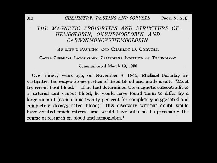
BOLD Endogenous Contrast • Blood Oxyenation Level Dependent Contrast – Deoxyhemoglobin is paramagnetic, oxyhemoglobin is less so. – Magnetic susceptibility of blood increases linearly with increasing oxygenation • Oxygen is extracted during passage through capillary bed – Arteries are fully oxygenated – Venous (and capillary) blood has increased proportion of deoxyhemoglobin – Difference between oxy and deoxy states is greater for veins BOLD sensitive to venous changes

Effects of TE and TR on T 2* Contrast MR Signal T 2 Decay T 1 Recovery 50 ms 1 s

Kwong et al. , 1992 VISUAL MOTOR
 in humans • Patterned visual")
Ogawa et al. , 1992 • High-field (4 T) in humans • Patterned visual stimulation at 10 Hz • Gradient-echo (GRE) pulse sequence used – Surface coil recorded • Significant image intensity changes in visual cortex • Image signal intensity changed with TE change – What form of contrast?

Blamire et al. , 1992 This was the first event-related f. MRI study. It used both blocks and pulses of visual stimulation. Gray Matter Hemodynamic response to long stimulus durations. Hemodynamic response to short stimulus durations. White matter Outside Head

Relation of BOLD Activity to Neuronal Activity

1. Information processing reflects collected neuronal activity • f. MRI response varies with pooled neuronal activity in a brain region – Behavior/cognitive ability determined by pooled activity • Alternatively, if single neurons governed behavior, f. MRI activation may be epiphenomenal
")
BOLD response reflects pooled local field potential activity (Logothetis et al, 2001)

f. MRI Hemodynamic Response Calcarine Sulci Fusiform Gyri 1500 ms 100 ms

Calcarine 1500 ms 100 ms Fusiform *

2. Co-localization • BOLD response reflects activity of neurons that are spatially co-localized • Based on what you know, is this true?

3. Measuring Deoxyhemoglobin • f. MRI measurements are of amount of deoxyhemoglobin per voxel • We assume that amount of deoxygenated hemoglobin is predictive of neuronal activity
 and Cerebral")
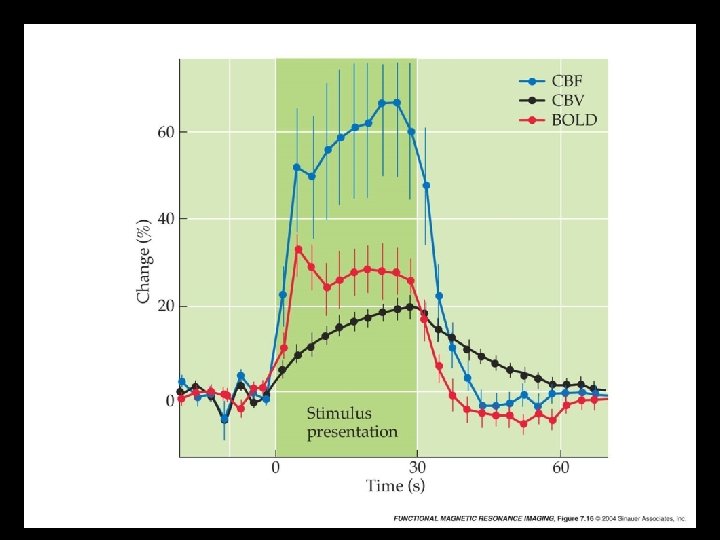
4. Uncoupling of CBF & CMRO 2 • Cerebral Blood Flow (CBF) and Cerebral Metabolic Rate of Oxygen (CMRO 2) are coupled under baseline conditions – PET measures CBF well, CMRO 2 poorly – f. MRI measures CMRO 2 well, CBF poorly • CBF about. 5 ml/g/min under baseline conditions – Increases to max of about. 7 -. 8 ml/g/min under activation conditions (+ 30%) • CMRO 2 only increases slightly with activation – May only increase by 10 -15% or less – Note: A large CBF change may be needed to support a small change in CMRO 2

The Hemodynamic Response

Impulse-Response Systems • Impulse: single event that evokes changes in a system – Assumed to be of infinitely short duration • Response: Resulting change in system Impulses Convolution Response = Output

Basic Form of Hemodynamic Response Peak Rise Initial Dip Baseline Undershoot Peak Sustained Response Rise Initial Dip Baseline Undershoot

Baseline Period • Why include a baseline period in epoch? – Corrects for scanner drift across time
 • Transient increase in oxygen consumption, before change in blood")
Initial Dip (Hypo-oxic Phase) • Transient increase in oxygen consumption, before change in blood flow – Menon et al. , 1995; Hu, et al. , 1997 • Shown by optical imaging studies – Malonek & Grinvald, 1996 • Smaller amplitude than main BOLD signal – 10% of peak amplitude (e. g. , 0. 1% signal change) • Potentially more spatially specific – Oxygen utilization may be more closely associated with neuronal activity than perfusion response

Early Evidence for the Initial Dip A C B Menon et al, 1995

Why is the initial dip controversial? • Not seen in most studies – Spatially localized to Minnesota – May require high field • Increasing field strength increases proportion of signal drawn from small vessels • Of small amplitude/SNR; may require more signal • Yacoub and Hu (1999) reported at 1. 5 T – May be obscured with large voxels or ROI analyses • May be selective for particular cortical regions – Yacoub et al. , 2001, report visual and motor activity • Mechanism unknown – Probably represents increase in activity in advance of flow – But could result from flow decrease or volume increase

Yacoub et al. , 2001

Negative BOLD response caused by impaired oxygen supply • Subject: 74 y male with transient ischemic attack (6 m prior) – Revealed to have arterial occlusion in left hemisphere • Tested in bimanual motor task • Found negative bold in LH, earlier than positive in right Rother, et al. , 2002
 • Results from vasodilation of arterioles, resulting in a large increase")
Rise (Hyperoxic Phase) • Results from vasodilation of arterioles, resulting in a large increase in cerebral blood flow • Inflection point can be used to index onset of processing

Peak – Overshoot • Over-compensatory response – More pronounced in BOLD signal measures than flow measures • Overshoot found in blocked designs with extended intervals – Signal saturates after ~10 s of stimulation

Sustained Response • Blocked design analyses rest upon presence of sustained response – Comparison of sustained activity vs. baseline – Statistically simple, powerful • Problems – Difficulty in identifying magnitude of activation – Little ability to describe form of hemodynamic response – May require detrending of raw time course

Undershoot • Cerebral blood flow more locked to stimuli than cerebral blood volume – Increased blood volume with baseline flow leads to decrease in MR signal • More frequently observed for longerduration stimuli (>10 s) – May not be present for short duration stimuli – May remain for 10 s of seconds


Issues in HDR Analysis • Delay in the HDR – Hemodynamic activity lags neuronal activity • Amplitude of the HDR • Variability in the HDR • HDR as a relative measure

The Hemodynamic Response Lags Neural Activity Experimental Design Convolving HDR Time-shifted Epochs Introduction of Gaps
 •")
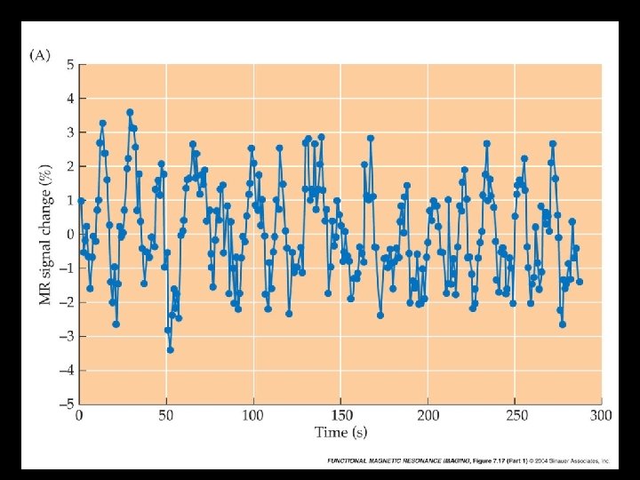
Percent Signal Change 505 1% 500 205 200 1% • Peak / mean(baseline) • Often used as a basic measure of “amount of processing” • Amplitude variable across subjects, age groups, etc.

Amplitude of the HDR • Peak signal change dependent on: – Brain region – Task parameters – Voxel size – Field Strength Kwong et al, 1992
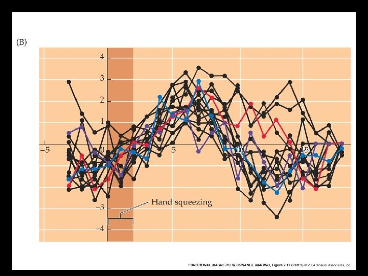

Variability in the Hemodynamic Response • • Across Subjects Across Sessions in a Single Subject Across Brain Regions Across Stimuli

Relative vs. Absolute Measures • f. MRI provides relative change over time – Signal measured in “arbitrary MR units” – Percent signal change over baseline • PET provides absolute signal – Measures biological quantity in real units • • CBF: cerebral blood flow CMRGlc: Cerebral Metabolic Rate of Glucose CMRO 2: Cerebral Metabolic Rate of Oxygen CBV: Cerebral Blood Volume

Spatial and Temporal Properties of BOLD f. MRI

Why do you need to know? • Spatial resolution – Trades off with coverage – Influences viability of preprocessing steps – Influences inferences about distinct ROIs • Temporal resolution – Tradeoffs between number of slices and TR – Needed resolution depends upon design

Spatial Resolution

What spatial resolution do we want? • Hemispheric – Lateralization studies – Selective attention studies • Systems / lobic – Relation to lesion data • Centimeter – Identification of active regions • Millimeter – Topographic mapping (e. g. , motor, vision) • Sub-millimeter – Ocular Dominance Columns – Cortical Layers

What determines Spatial Resolution? • Voxel Size – In-plane Resolution – Slice thickness • Spatial noise – Head motion – Artifacts • Spatial blurring – – Smoothing (within subject) Coregistration (within subject) Normalization (within subject) Averaging (across subjects)

Why can’t we just collect data from more/smaller voxels?

K – Space Revisited A . . . . . . B . . . FOV: 10 cm, Pixel Size: 2 cm FOV: 10 cm, Pixel Size: 1 cm To increase spatial resolution we need to sample at higher spatial frequencies.

Costs of Increased Spatial Resolution • Acquisition Time – In-plane • Higher resolution takes more time to fill K-space (resolution ~ size of K-space) – #Slices/second – Sample rates for 64*64 images • • Early Duke f. MRI: 2 -4 sl/s GE EPI: 12 sl/s Duke Spiral: 14 sl/s Duke Inverse Spiral: 21+ sl/s • Reduced signal per voxel – What is our dependent measure?

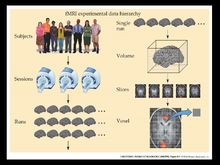
How large are functional voxels? 3. 75 mm 3. 75 m m 5. 0 mm = 3 ~. 08 cm Within a typical brain (~1300 cm 3), there may be about 20, 000 functional voxels.

How large are anatomical voxels? . 9 37 5 m m 5. 0 mm = 3 ~. 004 cm . 9375 mm Within a typical brain (~1300 cm 3), there may be about 300, 000+ anatomical voxels.

T 2* Blurring • Signal decays over time needed for collection of an image • For standard resolution images, this is not a critical issue • However, for high-resolution (in-plane) images, the time to acquire an image may be a significant fraction of T 2* • Under these conditions, multi-shot imaging may be necessary.

Partial Volume Effects • A single voxel may contain multiple tissue components – Many “gray matter” voxels will contain other tissue types – Large vessels are often present • The signal recorded from a voxel is a combination of all components

High Spatial Resolution f. MRI: Ocular Dominance Columns
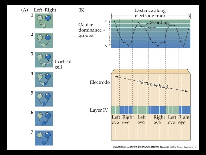

Early examples of ocular dominance Red = Left eye Blue = Right eye Pixel size 0. 5 mm 2 Menon et al. , 1997

Reliability of Ocular Dominance Measurements • Cheng et al. , 2001 • Same subject participated in two sessions – Raw data at left • Boundaries of dominance columns match well across sessions

Effects of Stimulus Duration on Spatial Extent of Activity

Example: Ocular Dominance Goodyear & Menon, 2001

4 sec 10 sec Goodyear & Menon, 2001

Example: Visual System 100 ms 500 ms 1500 ms
- Slides: 75