BMED 3520 Dynamic Continuous Models Book Chapter 4

Issue at Hand Hallmark Goals of Systems Biology: 1. Understand motifs and organizing principles 2. Design disease models for personalized medicine (1) Requires small models (math models: prove stuff) (2) Requires large models (computational models (Blue Brain): Wow!) Issue: All models require mathematical representations Where do we get these from? Before we address this question, let’s ask: Is a wrong model really so bad if it fits the data?

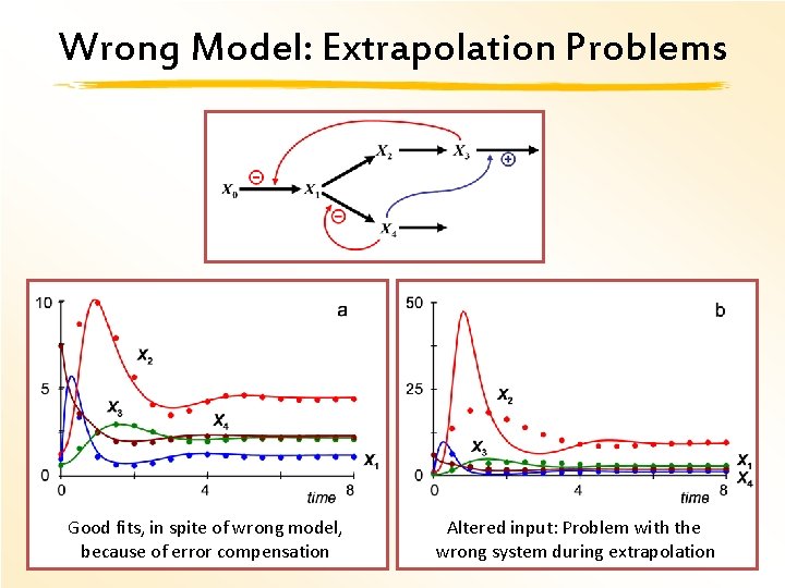
Wrong Model: Extrapolation Problems Good fits, in spite of wrong model, because of error compensation Altered input: Problem with the wrong system during extrapolation 3

True Representations … and Others Are there true representations: Probably not for realistic systems; why? Alternatives: 1. Make assumptions 2. Be oblivious to the issue; do what everybody else does (e. g. , SIR) 3. Use a sensible approximation Linear approximation (linearization) Nonlinear approximation 2 nd order Taylor approximation Canonical models

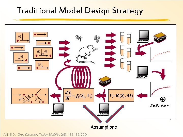
Traditional Model Design Strategy d. Xj = fk(Xj, Vi) dt Vi=Ri(Si, Mi) p 1, p 2, p 3, … 5 Assumptions Voit, E. O. : Drug Discovery Today Bio. Silico 2(5), 182 -189, 2004.

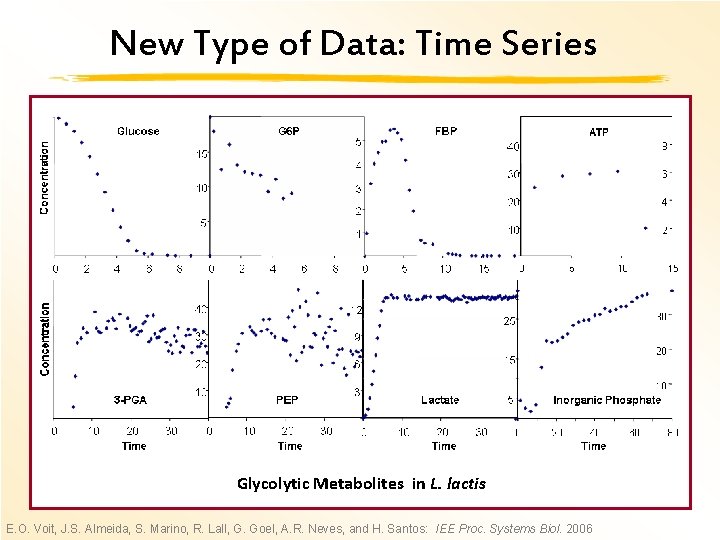
New Type of Data: Time Series Glycolytic Metabolites in L. lactis E. O. Voit, J. S. Almeida, S. Marino, R. Lall, G. Goel, A. R. Neves, and H. Santos: IEE Proc. Systems Biol. 2006

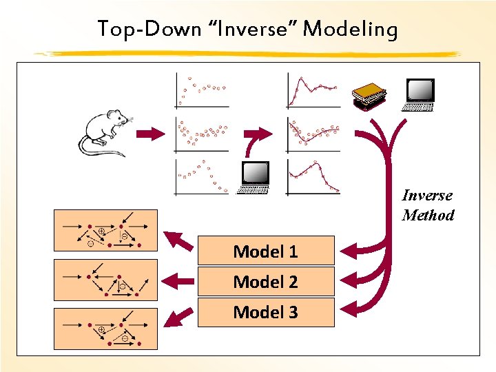
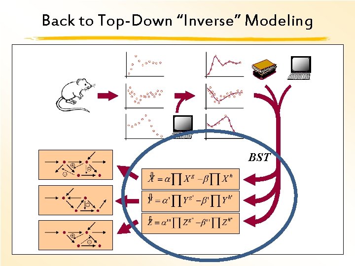
Top-Down “Inverse” Modeling Inverse Method Model 1 Model 2 Model 3 7

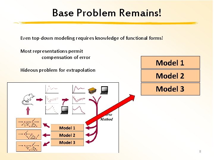
Base Problem Remains! Even top-down modeling requires knowledge of functional forms! Most representations permit compensation of error Hideous problem for extrapolation Model 1 Model 2 Model 3 8

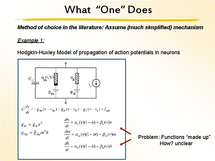
What “One” Does Method of choice in the literature: Assume (much simplified) mechanism Example 1: Hodgkin-Huxley Model of propagation of action potentials in neurons K Na Na K Problem: Functions “made up” How? unclear

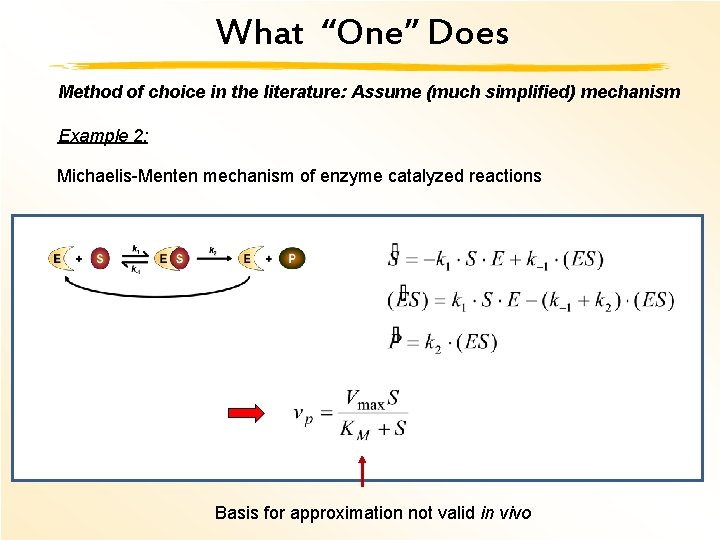
What “One” Does Method of choice in the literature: Assume (much simplified) mechanism Example 2: Michaelis-Menten mechanism of enzyme catalyzed reactions Basis for approximation not valid in vivo

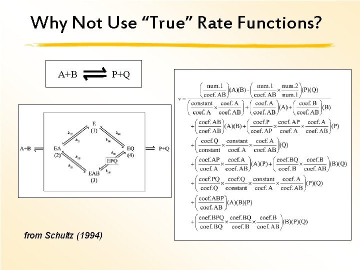
Why Not Use “True” Rate Functions? A+B from Schultz (1994) P+Q

Alternative: Approximation Replace complicated function with a simpler function How can we approximate a function if we don’t know it? Many approximations are possible Linear regression Are approximations valid? Do we have a choice? Aristotle (384 BC – 322 BC): “It is the mark of an educated mind to rest satisfied with the degree of precision which the nature of the subject admits and not to seek exactness where only an approximation is possible. ”

Alternative: Approximation Generic features: Operating Point (OP) [Note: nomenclature not always the same: OP = x, location on x-axis where F(x) is approximated OP = (x, F(x)), point where the approximation is anchored] Range of validity Brook Taylor (1715) proved that approximation is: perfect (at OP) great, good (close to OP) who knows? (far from OP)

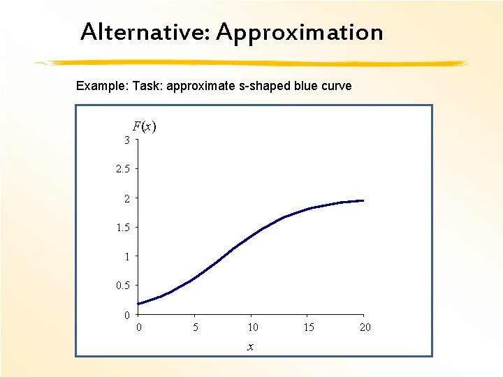
Alternative: Approximation Example: Task: approximate s-shaped blue curve 3 F(x) 2. 5 2 1. 5 1 0. 5 0 0 5 10 x 15 20

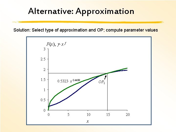
Alternative: Approximation Solution: Select type of approximation and OP; compute parameter values 3 F(x), g x f 2. 5 2 1. 5 0. 5323 x 0. 4499 OP 1 1 0. 5 0 0 5 10 x 15 20

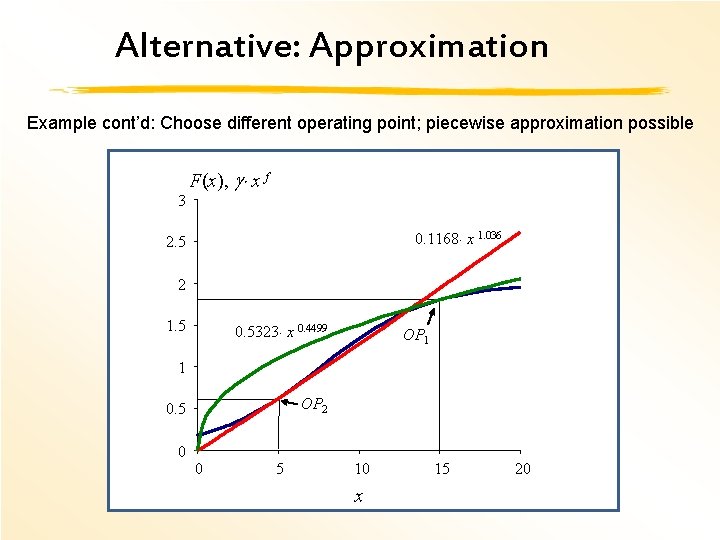
Alternative: Approximation Example cont’d: Choose different operating point; piecewise approximation possible 3 F(x), g x f 0. 1168 x 1. 036 2. 5 2 1. 5 0. 5323 x 0. 4499 OP 1 1 OP 2 0. 5 0 0 5 10 x 15 20

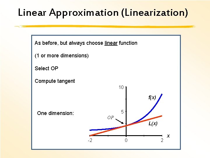
Linear Approximation (Linearization) As before, but always choose linear function (1 or more dimensions) Select OP Compute tangent 10 f(x) 5 One dimension: OP L(x) -2 0 2 x

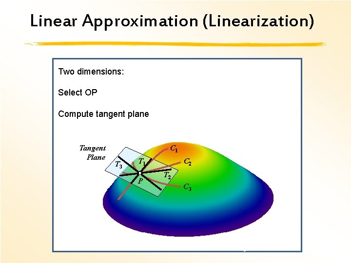
Linear Approximation (Linearization) Two dimensions: Select OP Compute tangent plane Tangent Plane C 1 T 3 T 1 P C 2 T 2 C 3

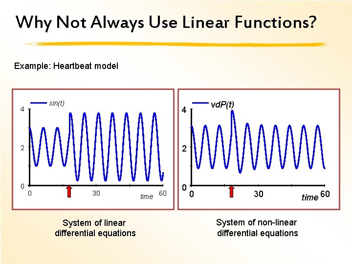
Why Not Always Use Linear Functions? Example: Heartbeat model sin(t) 4 2 2 0 vd. P(t) 4 0 30 System of linear differential equations time 60 0 0 30 System of non-linear differential equations time 60

Nonlinear Approximation Infinitely many nonlinear functions How to choose? Strategy 1: Use whatever seems to work Not very systematic Still need to choose Strategy 2: Canonical models

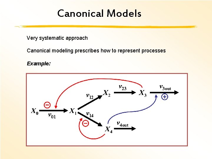
Canonical Models Very systematic approach Canonical modeling prescribes how to represent processes Example: v 12 v 01 v 23 v 14 v 4 out v 3 out

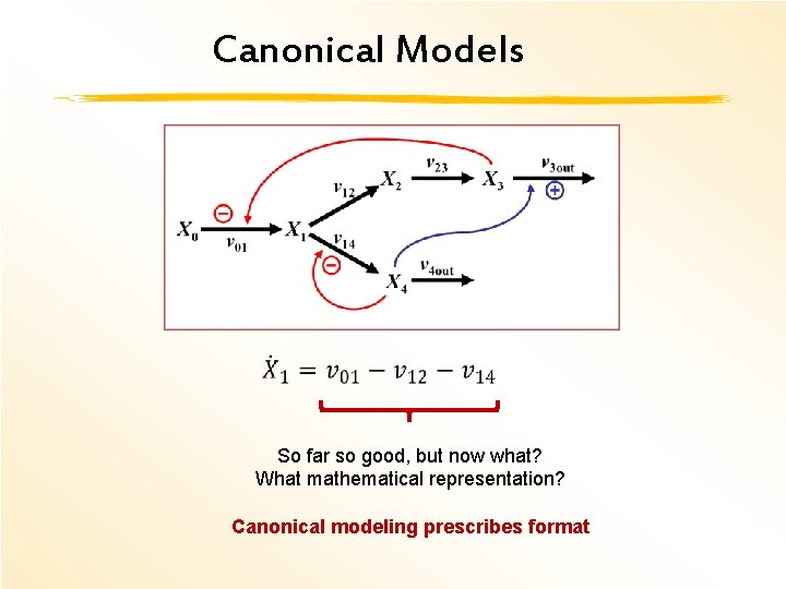
Canonical Models So far so good, but now what? What mathematical representation? Canonical modeling prescribes format

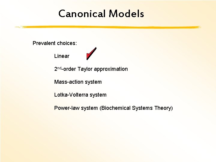
Canonical Models Prevalent choices: Linear 2 nd-order Taylor approximation Mass-action system Lotka-Volterra system Power-law system (Biochemical Systems Theory)

2 nd -Order Taylor Approximation Natural idea, but very inconvenient for large systems Especially messy for processes with many variables Seldom used in practice, except for one-dimensional problems

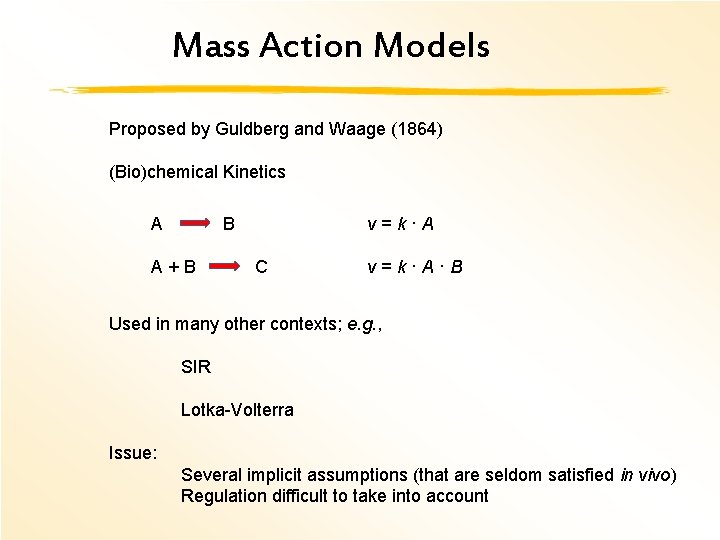
Mass Action Models Proposed by Guldberg and Waage (1864) (Bio)chemical Kinetics A B v = k · A A + B C v = k · A · B Used in many other contexts; e. g. , SIR Lotka-Volterra Issue: Several implicit assumptions (that are seldom satisfied in vivo) Regulation difficult to take into account

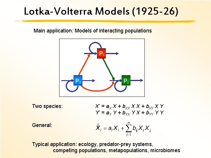
Lotka-Volterra Models (1925 -26) Main application: Models of interacting populations B 1 P B 3 P Two species: B 2 P X’ = a. X X + b. XX X X + b. XY X Y Y’ = a. Y Y + b. YX Y X + b. YY Y Y General: Typical application: ecology, predator-prey systems, competing populations, metapopulations, microbiomes

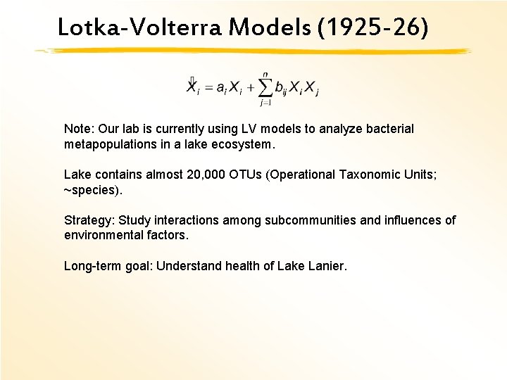
Lotka-Volterra Models (1925 -26) Note: Our lab is currently using LV models to analyze bacterial metapopulations in a lake ecosystem. Lake contains almost 20, 000 OTUs (Operational Taxonomic Units; ~species). Strategy: Study interactions among subcommunities and influences of environmental factors. Long-term goal: Understand health of Lake Lanier.

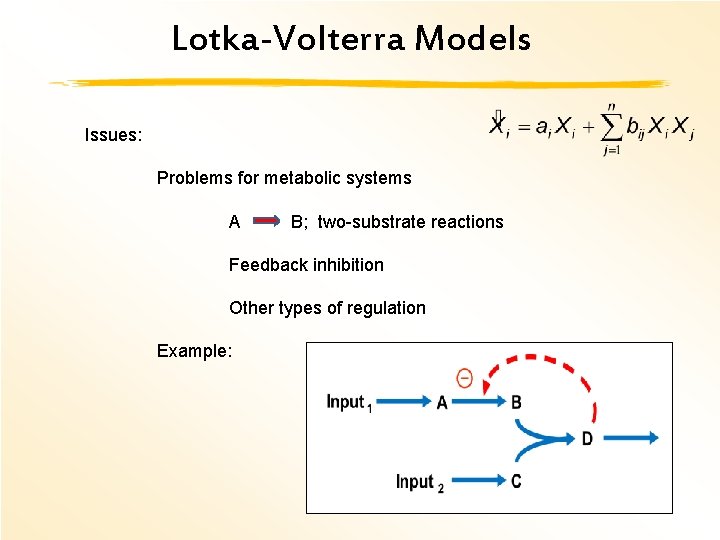
Lotka-Volterra Models Issues: Problems for metabolic systems A B; two-substrate reactions Feedback inhibition Other types of regulation Example:

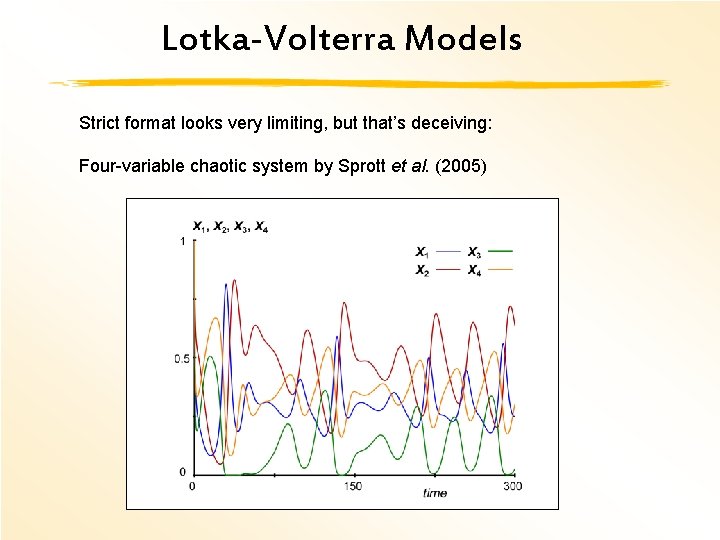
Lotka-Volterra Models Strict format looks very limiting, but that’s deceiving: Four-variable chaotic system by Sprott et al. (2005)

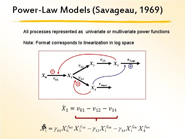
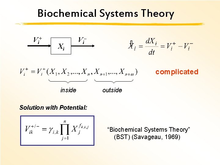
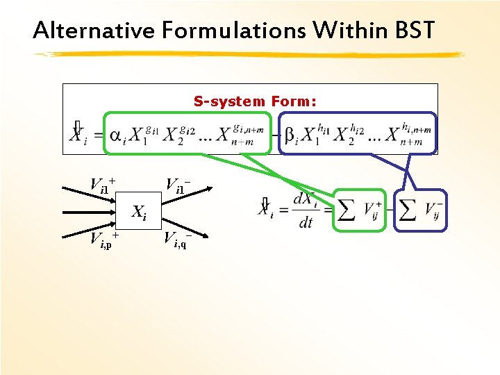
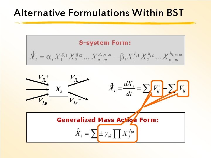
Power-Law Models (Savageau, 1969) All processes represented as univariate or multivariate power functions Note: Format corresponds to linearization in log space

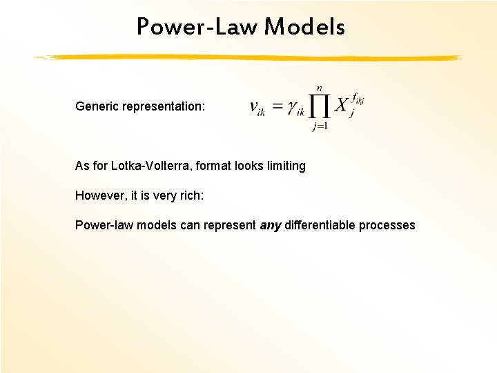
Power-Law Models Generic representation: As for Lotka-Volterra, format looks limiting However, it is very rich: Power-law models can represent any differentiable processes

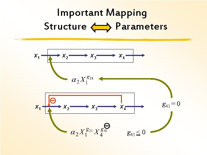
Important Mapping Structure Parameters X 1 X 2 X 3 X 4 g 41 = 0 g 41 < 0

Biochemical Systems Theory V i+ Xi V i– complicated inside outside Solution with Potential: “Biochemical Systems Theory” (BST) (Savageau, 1969)

Alternative Formulations Within BST S-system Form: Vi 1+ Vi 1– Xi Vi, p+ Vi, q–

Alternative Formulations Within BST S-system Form: Vi 1+ Vi 1– Xi Vi, p+ Vi, q– Generalized Mass Action Form:

Back to Top-Down “Inverse” Modeling BST 36

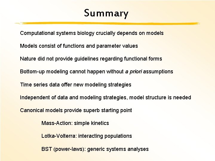
Summary Computational systems biology crucially depends on models Models consist of functions and parameter values Nature did not provide guidelines regarding functional forms Bottom-up modeling cannot happen without a priori assumptions Time series data offer new modeling strategies Independent of data and modeling strategies, model structure is needed Canonical models provide superb starting point Mass-Action: simple kinetics Lotka-Volterra: interacting populations BST (power-laws): generic systems analyses