Block Diagrams of Discrete Systems CSE 421 Digital

Block Diagrams of Discrete Systems CSE 421 Digital Control Lecture 6 1

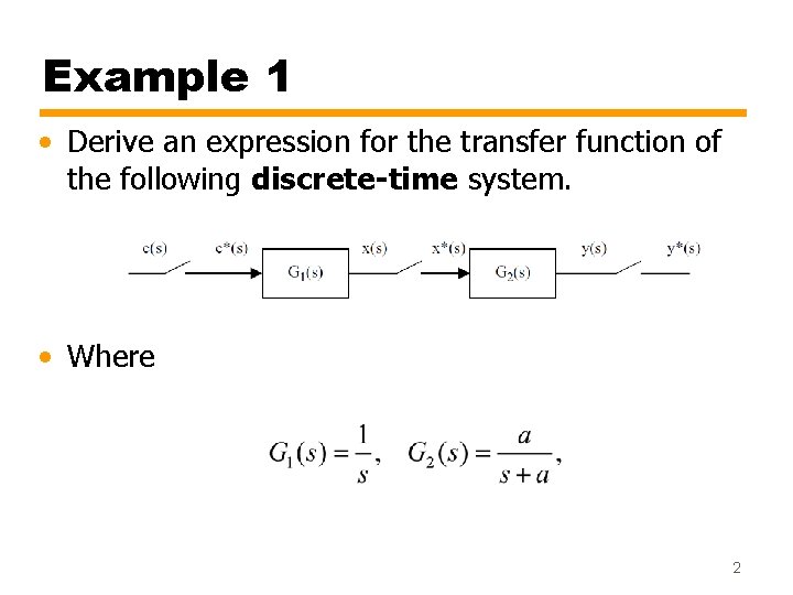
Example 1 • Derive an expression for the transfer function of the following discrete-time system. • Where 2

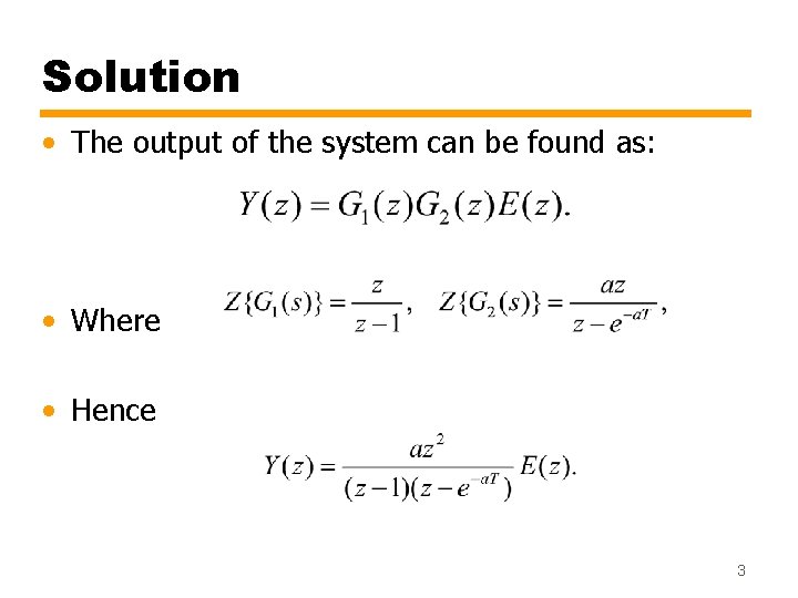
Solution • The output of the system can be found as: • Where • Hence 3

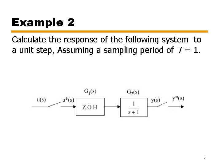
Example 2 Calculate the response of the following system to a unit step, Assuming a sampling period of T = 1. 4

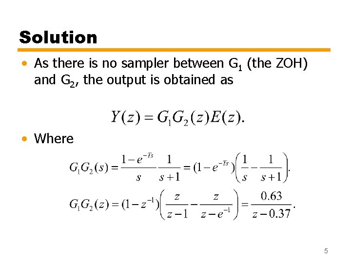
Solution • As there is no sampler between G 1 (the ZOH) and G 2, the output is obtained as • Where 5

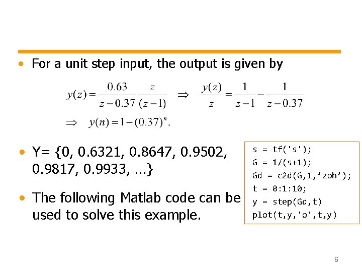
• For a unit step input, the output is given by • Y= {0, 0. 6321, 0. 8647, 0. 9502, 0. 9817, 0. 9933, …} • The following Matlab code can be used to solve this example. s = tf('s'); G = 1/(s+1); Gd = c 2 d(G, 1, ’zoh’); t = 0: 1: 10; y = step(Gd, t) plot(t, y, 'o', t, y) 6

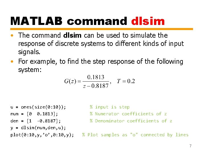
MATLAB command dlsim • The command dlsim can be used to simulate the response of discrete systems to different kinds of input signals. • For example, to find the step response of the following system: u = ones(size(0: 10)); num = [0 0. 1813]; den = [1 -0. 8187]; y = dlsim(num, den, u); plot(0: 10, y, ’o’, 0: 10, y); % input is step % Numerator coefficients of z % Denominator coefficients of z % Plot samples as "o" connected by lines 7

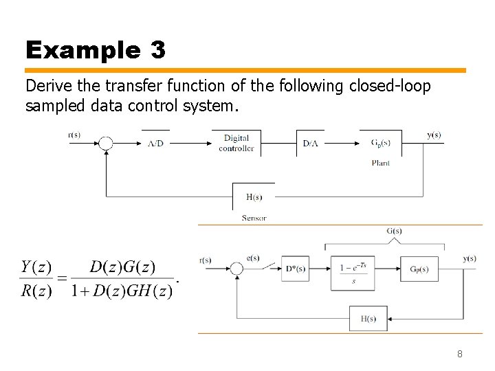
Example 3 Derive the transfer function of the following closed-loop sampled data control system. 8

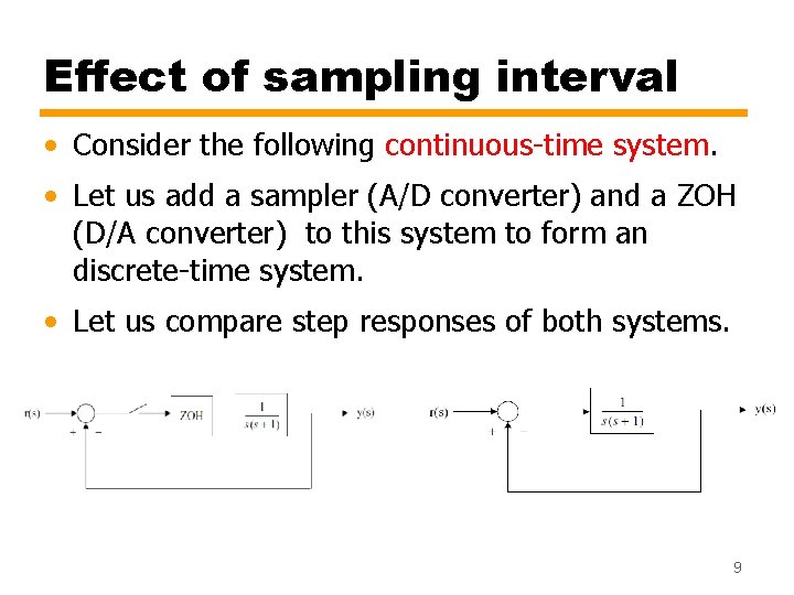
Effect of sampling interval • Consider the following continuous-time system. • Let us add a sampler (A/D converter) and a ZOH (D/A converter) to this system to form an discrete-time system. • Let us compare step responses of both systems. 9

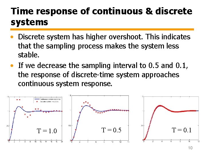
Time response of continuous & discrete systems • Discrete system has higher overshoot. This indicates that the sampling process makes the system less stable. • If we decrease the sampling interval to 0. 5 and 0. 1, the response of discrete-time system approaches continuous system response. T = 1. 0 T = 0. 5 T = 0. 1 10

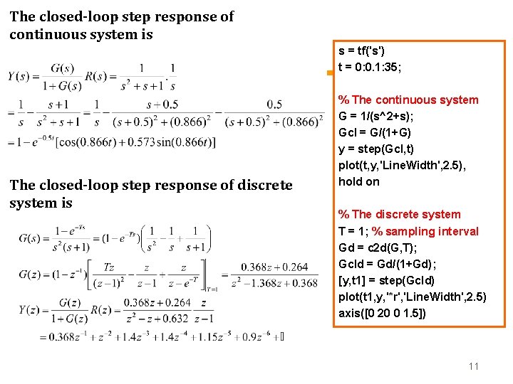
The closed-loop step response of continuous system is s = tf('s') t = 0: 0. 1: 35; The closed-loop step response of discrete system is % The continuous system G = 1/(s^2+s); Gcl = G/(1+G) y = step(Gcl, t) plot(t, y, 'Line. Width', 2. 5), hold on % The discrete system T = 1; % sampling interval Gd = c 2 d(G, T); Gcld = Gd/(1+Gd); [y, t 1] = step(Gcld) plot(t 1, y, '*r', 'Line. Width', 2. 5) axis([0 20 0 1. 5]) 11

Sample period selection • Large sampling interval has destabilizing effects on the system as the controller has no information about what is going on for the process output between samples. • In practice, a sampling interval of 1 second is short enough for e. g. pressure, temperature and flow control. • Faster electromechanical systems (e. g. motors) require much shorter sampling intervals in the order of milliseconds. • Some empirical rules for selecting sampling interval: - If the plant has dominant time constant τ, then choose sampling interval T < τ /10. - The sampling frequency should be 6 -20 times larger than the bandwidth of the plant. 12