Blind Source Separation PCA ICA HST 6 555

Blind Source Separation: PCA & ICA HST 6. 555 Gari D. Clifford gari@mit. edu http: //www. mit. edu/~gari © G. D. Clifford 2005

What is BSS? Assume an observation (signal) is a linear mix of >1 unknown independent source signals The mixing (not the signals) is stationary We have as many observations as unknown sources To find sources in observations - need to define a suitable measure of independence … For example - the cocktail party problem (sources are speakers and background noise):

The cocktail party problem - find Z z 1 x 1 z 2 x 2 A x. N XT=AZT z. N ZT XT

Formal statement of problem • N independent sources … Zmn ( M x. N ) • linear square mixing … Ann ( N x. N ) (#sources=#sensors) • produces a set of observations … Xmn ( M x. N ) …. . XT = AZT

Formal statement of solution • ‘demix’ observations … XT ( N x. M ) into YT = WXT YT ( N x. M ) ZT W ( N x. N ) A-1 How do we recover the independent sources? ( We are trying to estimate W A-1 ) …. We require a measure of independence!

‘Signal’ source ‘Noise’ sources Observed mixtures ZT XT=AZT YT=WXT

X Y = = A Z W X

The Fourier Transform (Independence between components is assumed)

Recap: non-Causal Wiener Filtering Observation Sx(f ) x[n] - observation Noise Power Sd(f ) y[n] - ideal signal d[n] - noise component Ideal Signal Sy(f ) Filtered signal: Sfilt (f ) = Sx(f ). H(f ) f

BSS is a transform? • Like Fourier, we decompose into components by transforming the observations into another vector space which maximises the separation between interesting (signal) and unwanted (noise). • Unlike Fourier, separation is not based on frequency- It’s based on independence • Sources can have the same frequency content • No assumptions about the signals (other than they are independent and linearly mixed) • So you can filter/separate in-band noise/signals with BSS

Principal Component Analysis • Second order decorrelation = independence • Find a set of orthogonal axes in the data (independence metric = variance) • Project data onto these axes to decorrelate • Independence is forced onto the data through the orthogonality of axes • Conventional noise/signal separation technique

Singular Value Decomposition Decompose observation X=AZ into…. X=USVT • S is a diagonal matrix of singular values with elements arranged in descending order of magnitude (the singular spectrum) • The columns of V are the eigenvectors of C=XTX (the orthogonal subspace … dot(vi, vj)=0 ) … they ‘demix’ or rotate the data • U is the matrix of projections of X onto the eigenvectors of C … the ‘source’ estimates

Singular Value Decomposition Decompose observation X=AZ into…. X=USVT

Eigenspectrum of decomposition • • • S = singular matrix … zeros except on the leading diagonal Sij (i=j) are the eigenvalues½ Placed in order of descending magnitude Correspond to the magnitude of projected data along each eigenvector Eigenvectors are the axes of maximal variation in the data [stem(diag(S). ^2)] Eigenspectrum= Plot of eigenvalues Variance = power (analogous to Fourier components in power spectra)

SVD noise/signal separation To perform SVD filtering of a signal, use a truncated SVD decomposition (using the first p eigenvectors) Y=USp. VT [Reduce the dimensionality of the data by discarding noise projections Snoise=0 Then reconstruct the data with just the signal subsapce] Most of the signal is contained in the first few principal components. Discarding these and projecting back into the original observation space effects a noise-filtering or a noise/signal separation

Two dimensional example

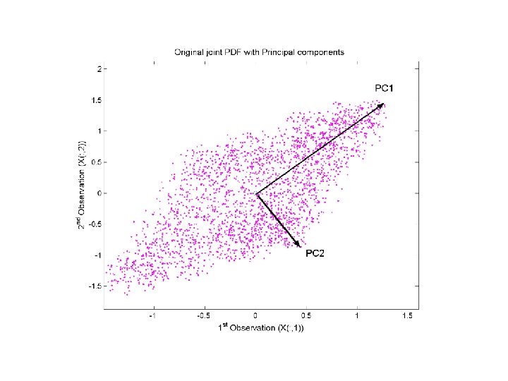
Real Data

Independent Component Analysis Like PCA, we are looking for N different vectors onto which we can project our observations to give a set of N maximally independent signals (sources) output data (discovered sources) dimensionality = dimensionality of observations Instead of using variance as our independence measure (i. e. decorrelating) as we do in PCA, we use a measure of how statistically independent the sources are.

The basic idea. . . Assume underlying source signals (Z ) are independent. Assume a linear mixing matrix (A )… XT=AZT in order to find Y ( Z ), find W, ( A-1 ). . . YT=WXT How? Initialise W & iteratively update W to minimise or maximise a cost function that measures the (statistical) independence between the columns of the YT.

Non-Gaussianity statistical independence? From the Central Limit Theorem, - add enough independent signals together, Sources, Z P(Z) ( <3 (1. 8) ) Mixtures (XT=AZT) P(X) ( =3. 4) Gaussian PDF ( =3)

Recap: Moments of a distribution

Higher Order Moments (3 rd -skewness) x

Higher Order Moments (4 th-kurtosis) Gaussians are mesokurtic with κ =3 Sub. Gaussian Super. Gaussian x

Entropy-based cost function Kurtosis is highly sensitive to small changes in distribution tails. A more robust measures of Gaussianity is based on differential entropy H(y), … negentropy: where ygauss is a Gaussian variable with the same covariance matrix as y. J(y) can be calculated from kurtosis … Entropy: measure of randomness- Gaussians are maximally random

Minimising Mutual Information Mutual information (MI) between two vectors x and y : I = Hx + Hy - Hxy always non-negative and zero if variables are independent … therefore we want to minimise MI. MI can be re-written in terms of negentropy … where c is a constant. … differs from negentropy by a constant and a sign change

Measures of Statistical Independence In general we require a measure of statistical independence which we maximise between each of the N components. Non-Gaussianity is one approximation, but sensitive to small changes in the distribution tail. Other measures include: • Mutual Information I, • Entropy (Negentropy, J )… and • Maximum (Log) Likelihood

Independent source discovery using Maximum Likelihood Generative latent variable modeling N observables, X. . . from N sources, zi through a linear mapping W=wij Latent variables assumed to be independently distributed Find elements of W by gradient ascent - iterative update by where is some learning rate (const) … and is our objective cost function, the log likelihood

Weight updates W=[1 3; -2 -1] wij Iterations/100

The Cocktail Party Problem Revisited … some practical examples using ICA

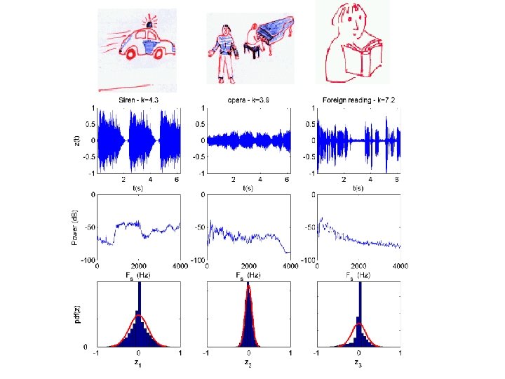
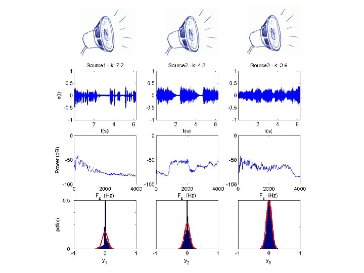
Observations Separation of mixed observations into source estimates is excellent … apart from: • Order of sources has changed • Signals have been scaled Why? … In XT=AZT, insert a permutation matrix B … XT=ABB-1 ZT … = sources with different col. order. sources change by a scaling A AB … ICA solutions are order and scale independent because κ is dimensionless & measured between the sources … - It is a relative measure between the outputs.

Separation of sources in the ECG

=3 =11 =0 =3 =1 =5 =0 =1. 5

Transformation inversion for filtering • Problem - can never know if sources are really reflective of the actual source generators - no gold standard • De-mixing might alter the clinical relevance of the ECG features • Solution: Identify unwanted sources, set corresponding (p) columns in W-1 to zero (Wp-1 ), then multiply back through to remove ‘noise’ sources and transform back into original observation space.

Transformation inversion for filtering

Real Data X Y=WX Z Xfilt = Wp-1 Y

ICA results 4 X Y=WX Z Xfilt = Wp-1 Y

Summary • PCA is good for Gaussian noise separation • ICA is good for non-Gaussian ‘noise’ separation • PCs have obvious meaning - highest energy components • ICA - derived sources : arbitrary scaling/inversion & ordering …. need energy-independent heuristic to identify signals / noise • Order of ICs change - IC space is derived from the data. - PC space only changes if SNR changes. • ICA assumes linear mixing matrix • ICA assumes stationary mixing • De-mixing performance is function of lead position • ICA requires as many sensors (ECG leads) as sources • Filtering - discard certain dimensions then invert transformation • In-band noise can be removed - unlike Fourier!