Blind SearchPart 2 Ref Chapter 2 Search Trees

Blind Search-Part 2 Ref: Chapter 2

Search Trees • The search for a solution can be described by a tree - each node represents one state. • The path from a parent node to a child node represents an operation. • Search Trees provide a convenient description of the search space, they are not a data structure stored in memory!!!

Search Trees • Each node is a search tree has child nodes that represent each of the states reachable by the parent state. • Another way of looking at it: child nodes represent all available options once the search procedure reaches the parent node. • There a number of strategies for traversing a search tree.

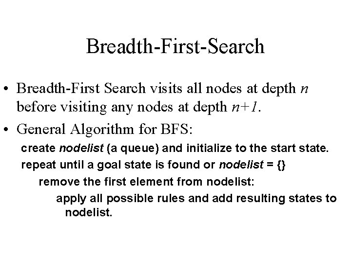
Breadth-First-Search • Breadth-First Search visits all nodes at depth n before visiting any nodes at depth n+1. • General Algorithm for BFS: create nodelist (a queue) and initialize to the start state. repeat until a goal state is found or nodelist = {} remove the first element from nodelist: apply all possible rules and add resulting states to nodelist.

Breadth-First Search Characteristics • If there is a solution, BFS will find it. • BFS will find the minimal solution (shortest path length to the solution). • BFS will not get caught in state space cycles. • Requires space available to store the nodelist queue. This can be very large!!!

BFS Time and Space Analysis • Assumptions: – There is a single solution (goal state) in the tree. – The search tree is “regular” and has branching factor b. – The goal state is at depth d in the tree. – The goal state is in the middle of the tree (average case analysis).

BFS Space Requirements • The queue initially has 1 state. • After the first step - the queue will contain b states. • Processing each of the b states at level 1 results in adding b more states to the queue. • After processing all states at depth n, the queue will hold bn-1 states.

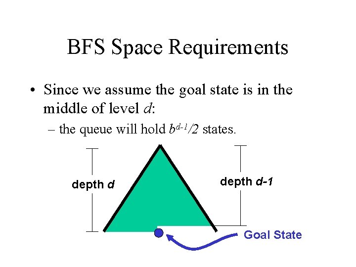
BFS Space Requirements • Since we assume the goal state is in the middle of level d: – the queue will hold bd-1/2 states. depth d-1 Goal State

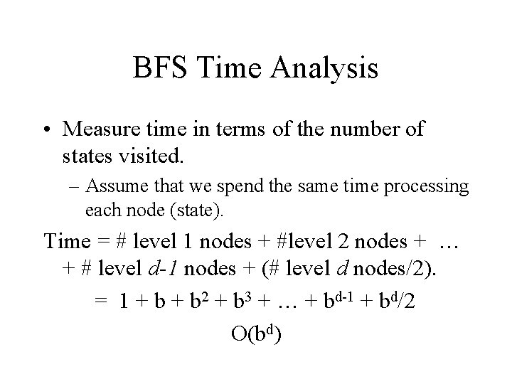
BFS Time Analysis • Measure time in terms of the number of states visited. – Assume that we spend the same time processing each node (state). Time = # level 1 nodes + #level 2 nodes + … + # level d-1 nodes + (# level d nodes/2). = 1 + b 2 + b 3 + … + bd-1 + bd/2 O(bd)

Depth-First Search Depth-First processes all children (choices) of a node before considering any siblings (at the same depth). Depth-First Search is similar to BFS, but instead of a queue we use a stack. Depth-First Search can easily be described recursively.

DFS recursive definition While applicable rules exist: apply the next rule and generate a new state. If new state is the goal - all done, Otherwise - do a depth-first search on the new state.

DFS • General Algorithm for DFS: create nodelist (a stack) and initialize to the start state. repeat until a goal state is found or nodelist = {} pop the first element from nodelist: apply all possible rules and add (push) resulting states to nodelist.

DFS Space Analysis • After the first step the stack will contain b nodes. • After the second step the stack will contain (b - 1) + b nodes. • After the 3 rd step the stack will contain (b 1) + (b-1) + b nodes. • After the first d steps the stack will hold (b 1)*d + 1 nodes (this is the maximum).

DFS Time Analysis • In the best case - the goal state will be the first state examined at depth d - this will require looking at d+1 nodes. • In the worst case - the goal state will be the last state examined at depth d - this will require looking at all the nodes: 1+b+b 2+b 3+…+bd = (bd+1 -1) / (b-1)

DFS average time • Not as obvious how to calculate the average time as it was with BFS. • Book goes through a derivation, the point is that DFS is also O(bd) in the average case.

Depth-First Search Characteristics • Don’t need to keep track of a large list of states. • May find a solution very fast (and might not). • “Pruning” is possible – example: branch-and-bound • Can easily get caught in loops.

Iterated Deepening • Attempt to combine BFS and DFS to get a search with the following desirable characteristics: – Find the minimal solution (shortest path length to the solution). – Minimal (reasonable) space requirements – Similar time requirements.

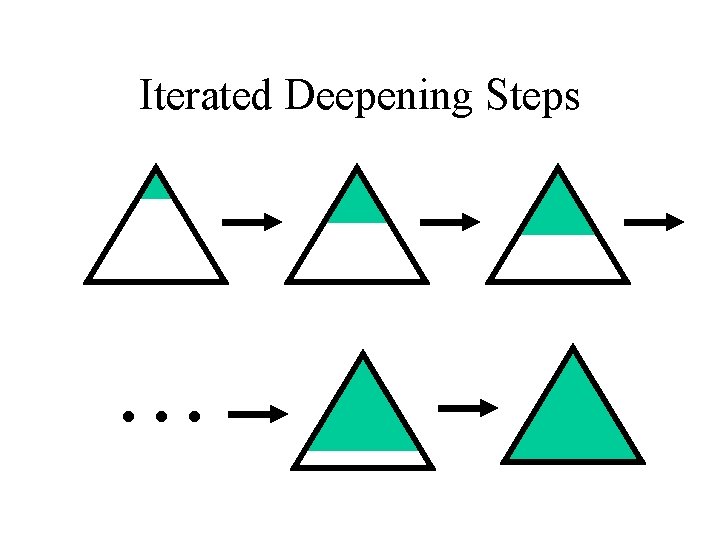
Iterated Deepening • Iterated Deepening uses a depth cutoff that starts at depth 1. • For each depth cutoff 1. . d do: – apply DFS stopping at the cutoff depth. – If goal state is not found increase the depth cutoff.

Iterated Deepening Steps . . .

Iterated Deepening Analysis • Maximum space requirements is the same as DFS: O(bd) • Worst case/Average case time analysis: O(1 + b 2 + b 3 + … + bd) O(bd)

Iterated Broadening • Limit on the breadth of a search at each node (number of child nodes processed). • Gradually increase the breadth limit until a goal is found. • Iterated broadening is most useful when there are many goals in the search tree.

Iterated Broadening Time Analysis • At most we must run b searches (each with different breadth cutoff). • First search includes 1 node. • Second search looks at 2 d • Third looks at 3 d • … 1+2 d+3 d+…+bd => O(bd)

Loops • DFS (and iterated deepening) can suffer if there are loops in the state space. • In problems that can generate loops we need to treat the search space as a graph. • There a number of modifications that are possible

Searching Graphs • The general idea is to keep track of all nodes that have already been searched. • Each time a new node is put on the stack/queue we first make sure it has not already been processed. • The list of nodes already processed is called the “closed list” and the stack/queue is called the “open list”.

Problems with using Closed List • The closed list can (and will) become too large. • It takes time O(|Closed List|) to make sure each new node has not already been processed. • Possible solutions: – Use hash tables – Limit the size of the Closed List?