Blending Surfaces Introduction Blending n 1 The act

Blending Surfaces
 The")
Introduction Blending n. 1. The act of mingling. 1913 Webster 2. (Paint. ) The method of laying on different tints so that they may mingle together while wet, and shade into each other insensibly. --Weale. 1913 Webster

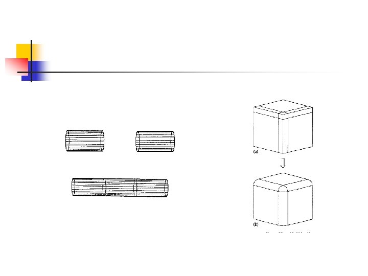
Introduction n n The process of mixing several base objects to form a new object. The process of providing smooth transition between intersecting surfaces or smooth connection between disjoint surfaces.

A General Blending model n We have seen a Belnding method before ! (where ? ) Lets presents a simple scheme for point blending:

A General Blending Model n n n Bezier and Bspline representation is exactly of this form. Q. Why use Points as the Base objects? A. There is no reason

A General Blending Model n n Let Q be an arbitrary parametrically defined objects. The general parametric equation is we receive is: Q – base objects b – blending functions

Blending example n n n Blending a set of curves for example: We use a continues function b which satisfy the following conditions: Then blending and , two parametric curves on the same domain is:

Blending example n n n We can immediately see that: S is a surface. S(0, t) is a curve. (which one ? ) S(1, t) is a curve. (which one ? ) Q. Can we blend in this way surfaces ? A. Yes

Blending Function n We will use the Bernstein functions to create a smooth blending function. Let be the i-th Bernstein basis function of degree n. lets define :

Blending functions

General Equation n Let S 1 and S 2 be two smooth surfaces then we can define:

Rail curves n S is a blending surface smoothly connecting S 1 and S 2 along the rail curves S 1(0, t) , S 2(1, t)

The intersection problem n n n Finding the intersection curve between two surfaces is a Hard problem. Algebraic solutions – complex , good for low dimensionality. Numerically solutions – not accurate, loose parameterization.

The intersection problem n n Solution: Numerically find points on the intersection curve. Construct a curve C that interpolate the points. Locally change the surfaces so they pass through C.
 be a smooth curve on [c,")
Curve/Surface Blending Model n n n Let c(t) be a smooth curve on [c, d] S 1(s, t) a smooth surface on [a, b]X[c, d] We define:

Blending function

Curve / Surface Blending Model n The new parametric surface we get is:

Curve / Surface Blending n n We can easily see that the interpolated curve pass through the new Surface. To finish the algorithm we will use the model presented earlier on our problem.
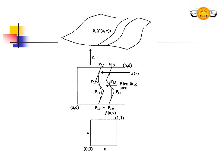
 is a curve defined on [a,")
Curve / Surface Blending n n n C(t) is a curve defined on [a, b] S 1(s, t) is a surface defined on [a, b]x[c, d] C 1=S 1(h(v)) a curve on S 1 h(v) is a function from [0, 1] to [a, b]X[c, d] For simplicity:

Curve / Surface Blending n n We need to create a blending erea. This is done by sweeping h(v) to the right. And the blending area is:

Curve / Surface Blending n Thus the blending surface is:

surfaces – 2 curves 3 n n Can we use a similar approach for more variables ? Yes we can …

Surface/Surface – Corner Blending

Surface/Surface – Corner Blending n Blending is done in the parameter space. n Intersection curve can be approximated !

Blending functions

Constructing b definitions 1 n n Bernstein of degree 5 f- mapping (rotation / translation)
 = Bernstein triangular Edges are bizier curves.")
Bernstein triangular n n n C(s, t) = Bernstein triangular Edges are bizier curves. Fits our parameters (c 1)

Blending function
 , Q(s, t)")
Blend by pointwise interpolation n n Given two surfaces P(u, v) , Q(s, t) Let A(w) , B(w) two respective contact curves: A(w)=P(u(w), v(w)) B(w)=Q(s(w), t(w)) We pick two vectors in the tangent plane.

pointwise interpolation n A general form of the vectors:

pointwise interpolation n Using global functions M 0 and M 1 :

Blend by pointwise interpolation n And the new surface is:

Choices of functions n n n There are many choices for M and N. Tangent vectors T are more application driven. Example:

Geometric correspondence n n Hard problem There is No good solution.

Fanout surface technique n Using intrinsic properties of the curves !
")
Fanout surface technique n If P is a point on A. (the contact curve) And the curve becomes:

The fanout surface n Using a and p as parameters gives us the fanout surface: And in a similar way:

Funout surfaces intersection n n The intersection of the fanout surfaces gives us the needed correspondence. 3 equations , 4 unknowns, one parameter Q. Where are the 3 equations? A. Next page…

Correspondence solution
 , p=p(w) , b=b(w) , q=q(w) We have a")
Correspondence solution n n a=a(w) , p=p(w) , b=b(w) , q=q(w) We have a parametric solution from degree 1 = curve !

THE END n
- Slides: 43