Biplot Analysis of MultiEnvironment Trial Data Weikai Yan

Biplot Analysis of Multi-Environment Trial Data Weikai Yan May 2006 Contact: wyan@ggebiplot. com

Multi-Environment Trials (MET) • • MET are essential MET are expensive MET data are valuable MET data are not fully used Weikai Yan 2006

Why biplot analysis? • Biplot analysis can help understand MET data – Graphically, – Effectively, – Conveniently Weikai Yan 2006

Outline • • • Multi-environment trial (MET) data Basics of biplot analysis Biplot analysis of G-by-E data Biplot analysis of G-by-T data Better understanding of MET data Conclusions Weikai Yan 2006

Multi-environment trial data Contact: wyan@ggebiplot. com

MET data is a genotype-environment-trait (G-E-T) 3 -way table • Multiple Genotypes • Multiple Environments • Multiple Traits Weikai Yan 2006

A G-E-T 3 -way table contains many 2 -way tables • G by E: for each trait • G by T (trait): in each environment; across environments • E by T: for each genotype; across genotypes G-E-T data >> G-E data Weikai Yan 2006

A G-E-T 3 -way table is an extended 2 -way table • G by V: – each E-T combination as a variable (V) • P by T: – each G-E combination as a phenotype (P) Weikai Yan 2006

A G-E-T 3 -way table implies informative 2 -way tables • Association by environment 2 -way tables – Associations: • among traits • between traits and genetic markers Weikai Yan 2006

Goals of MET data analysis • Short-term goals: – Variety evaluation • Response to the environment (G x E) • Trait profiles (G x T) • Long-term goals: – To understand • • the target environment (G x E) the test environments (G x E) the crop (G x T) the genotype x environment interaction (A x T) Weikai Yan 2006

Basics of biplot analysis Most two-way tables can be visually studied using biplots Contact: wyan@ggebiplot. com

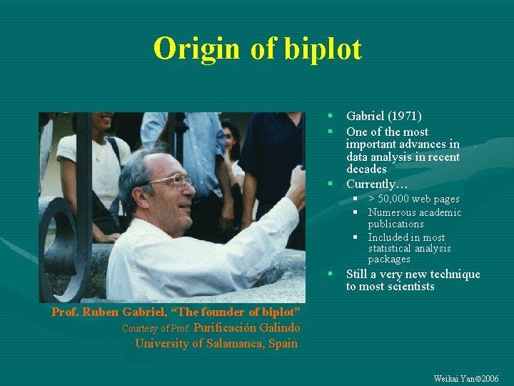
Origin of biplot § § § Gabriel (1971) One of the most important advances in data analysis in recent decades Currently… § > 50, 000 web pages § Numerous academic publications § Included in most statistical analysis packages § Still a very new technique to most scientists Prof. Ruben Gabriel, “The founder of biplot” Courtesy of Prof. Purificación Galindo University of Salamanca, Spain Weikai Yan 2006

What is a biplot? • “Biplot” = “bi” + “plot” – “plot” • scatter plot of two rows OR of two columns, or • scatter plot summarizing the rows OR the columns – “bi” • BOTH rows AND columns • 1 biplot >> 2 plots Weikai Yan 2006

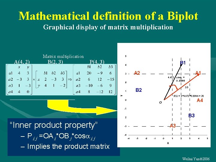
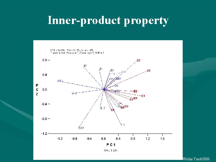
Mathematical definition of a Biplot Graphical display of matrix multiplication A(4, 2) Matrix multiplication B(2, 3) P(4, 3) B 1 A 2 A 1 4. 472 cos = 0. 8944 5. 0 B 2 P 11 = 5*4. 472*0. 8944 = 20 A 4 B 3 “Inner product property” A 3 – Pij =OAi*OBj*cos ij – Implies the product matrix Weikai Yan 2006

Practical definition of a biplot “Any two-way table can be analyzed using a 2 D-biplot as soon as it can be sufficiently approximated by a rank-2 matrix. ” (Gabriel, 1971) (Now 3 D-biplots are also possible…) Matrix decomposition P(4, 3) G(3, 2) E 1 E(2, 3) G 2 G 1 E 2 G 4 G-by-E table E 3 G 3 Weikai Yan 2006

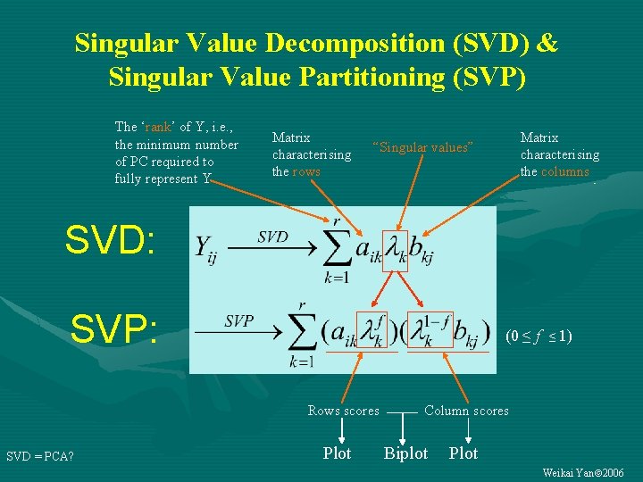
Singular Value Decomposition (SVD) & Singular Value Partitioning (SVP) The ‘rank’ of Y, i. e. , the minimum number of PC required to fully represent Y Matrix characterising the rows Matrix characterising the columns “Singular values” SVD: SVP: (0 ≤ f ≤ 1) Rows scores SVD = PCA? Plot Column scores Biplot Plot Weikai Yan 2006

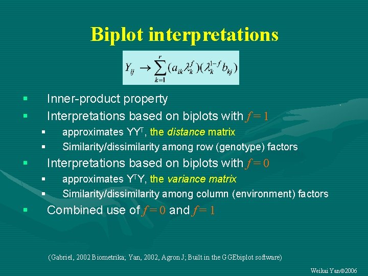
Biplot interpretations § § Inner-product property Interpretations based on biplots with f = 1 § § § Interpretations based on biplots with f = 0 § § § approximates YYT, the distance matrix Similarity/dissimilarity among row (genotype) factors approximates YTY, the variance matrix Similarity/dissimilarity among column (environment) factors Combined use of f = 0 and f = 1 (Gabriel, 2002 Biometrika; Yan, 2002, Agron J; Built in the GGEbiplot software) Weikai Yan 2006

Biplot analysis is… to use biplots to display – a two-way data per se (Y), – its distance matrix (YYT), and – its variance matrix (YTY) so that – relationships among rows, – relationships among columns, and – interactions between rows and columns can be graphically visualized. Weikai Yan 2006

Data centering prior to biplot analysis • The general linear model for a G-by-E data set (P) – P = M + G + E + GE • Possible two-way “tables” (Y): • • • Y = P = M + G + E + GE —original data: QQE biplot Y = P – M = G + E + GE —global-centered (PCA) Y = P – M – E = G + GE —column-centered: GGE biplot Y = P – M – G = E + GE —row-centered Y = P – M – G – E = GE —double-centered: GE biplot All models are useful, depending on the research objectives (built in GGEbiplot) Weikai Yan 2006

Data scaling prior to biplot analysis • Different GGE biplots • Yij = ( i + ij)/sj • Sj = 1 • Sj = (s. d. )j • Sj = (s. e. )j no scaling all environments are equally important heterogeneity among environments is removed (built in GGEbiplot) Weikai Yan 2006

Four questions must be asked before trying to interpret a biplot 1. What is the model? How the data were centered and scaled? What are we looking at? 2. What is the goodness of fit? How confident are we about what we see? What if the data is fitted poorly? 3. How singular values are partitioned? What questions can be asked? 4. Are the axes drawn to scale? Are the patterns artifacts? (All are addressed explicitly in GGEbiplot) Weikai Yan 2006

Biplot Analysis of G-by-E data GENOTYPE EVALUATION TEST ENVIRONMENT EVALUATION MEGAENVIRONMENT ANALYSIS Contact: wyan@ggebiplot. com

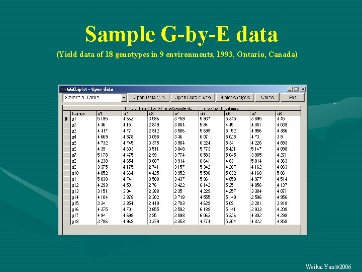
Sample G-by-E data (Yield data of 18 genotypes in 9 environments, 1993, Ontario, Canada) Weikai Yan 2006

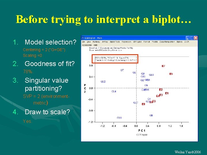
Before trying to interpret a biplot… 1. Model selection? Centering = 2 (“G+GE”) Scaling =0 2. Goodness of fit? 78%. 3. Singular value partitioning? SVP = 2 (environmentmetric) 4. Draw to scale? Yes. Weikai Yan 2006

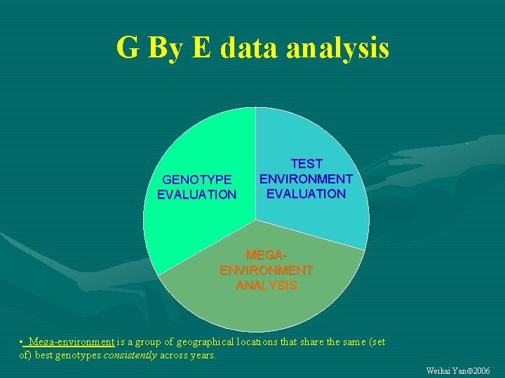
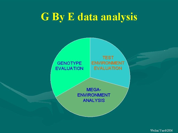
G By E data analysis GENOTYPE EVALUATION TEST ENVIRONMENT EVALUATION MEGAENVIRONMENT ANALYSIS • Mega-environment is a group of geographical locations that share the same (set of) best genotypes consistently across years. Weikai Yan 2006

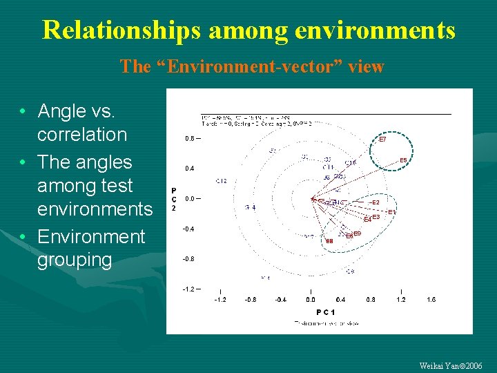
Relationships among environments The “Environment-vector” view • Angle vs. correlation • The angles among test environments • Environment grouping Weikai Yan 2006

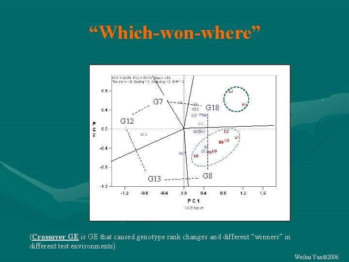
“Which-won-where” G 7 G 18 G 12 G 13 G 8 (Crossover GE is GE that caused genotype rank changes and different “winners” in different test environments) Weikai Yan 2006

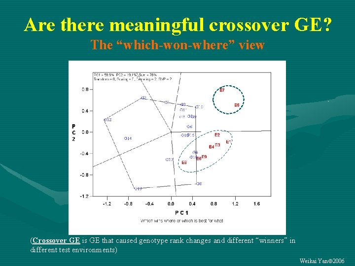
Are there meaningful crossover GE? The “which-won-where” view (Crossover GE is GE that caused genotype rank changes and different “winners” in different test environments) Weikai Yan 2006

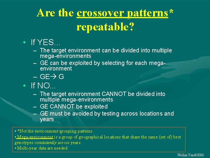
Are the crossover patterns* repeatable? • If YES… – The target environment can be divided into multiple mega-environments – GE can be exploited by selecting for each megaenvironment – GE G • If NO… – The target environment CANNOT be divided into multiple mega-environments – GE CANNOT be exploited – GE must be avoided by testing across locations and years • *Not the environment-grouping patterns • Mega-environment is a group of geographical locations that share the same (set of) best genotypes consistently across years. • Multi-year data are needed Weikai Yan 2006

Classify your target environment into one of three categories Repeatable With Crossover GE No Crossover GE (2) Multiple MEs (1) Single simple ME Select for specifically adapted genotypes for each ME Not repeatable (3) Single complex ME A single test location, single year suffices to select a single best variety Select for generally adapted genotypes across the whole regions across multiple years ME: mega-environment Weikai Yan 2006

G By E data analysis GENOTYPE EVALUATION TEST ENVIRONMENT EVALUATION MEGAENVIRONMENT ANALYSIS Weikai Yan 2006

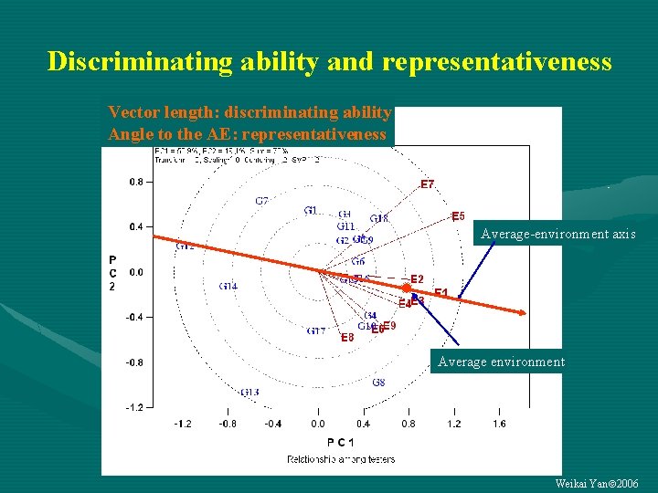
Discriminating ability and representativeness Vector length: discriminating ability Angle to the AE: representativeness Average-environment axis Average environment Weikai Yan 2006

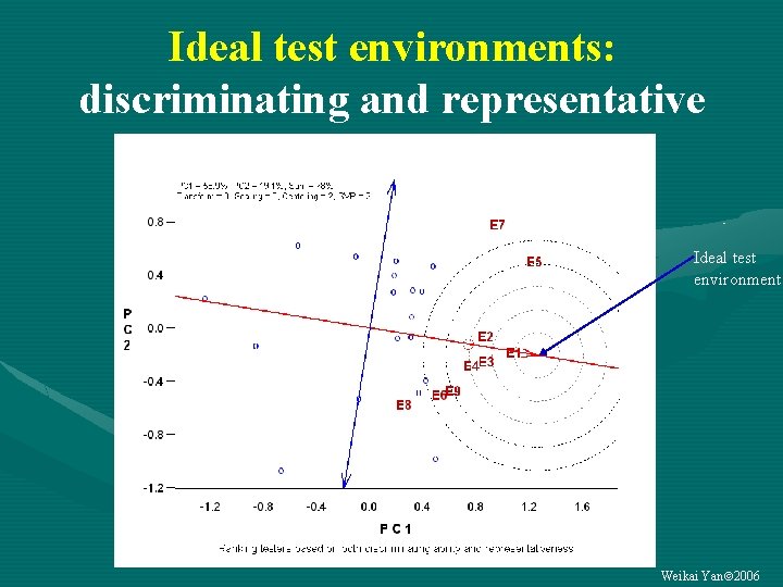
Ideal test environments: discriminating and representative Ideal test environment Weikai Yan 2006

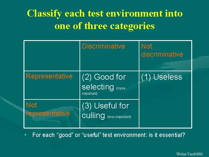
Classify each test environment into one of three categories Representative Discriminative Not discriminative (2) Good for selecting (more (1) Useless important) Not representative (3) Useful for culling (less important) • For each “good” or “useful” test environment: is it essential? Weikai Yan 2006

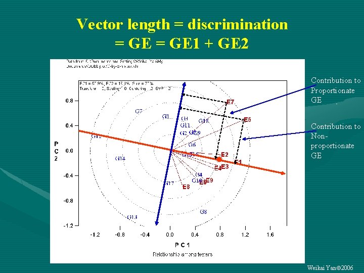
Vector length = discrimination = GE 1 + GE 2 Contribution to Proportionate GE Contribution to Nonproportionate GE Weikai Yan 2006

G By E data analysis GENOTYPE EVALUATION TEST ENVIRONMENT EVALUATION MEGAENVIRONMENT ANALYSIS Weikai Yan 2006

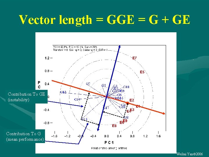
Vector length = GGE = G + GE Contribution To GE (instability) Contribution To G (mean performance) Weikai Yan 2006

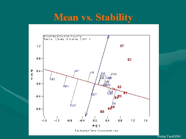
Mean vs. Stability Weikai Yan 2006

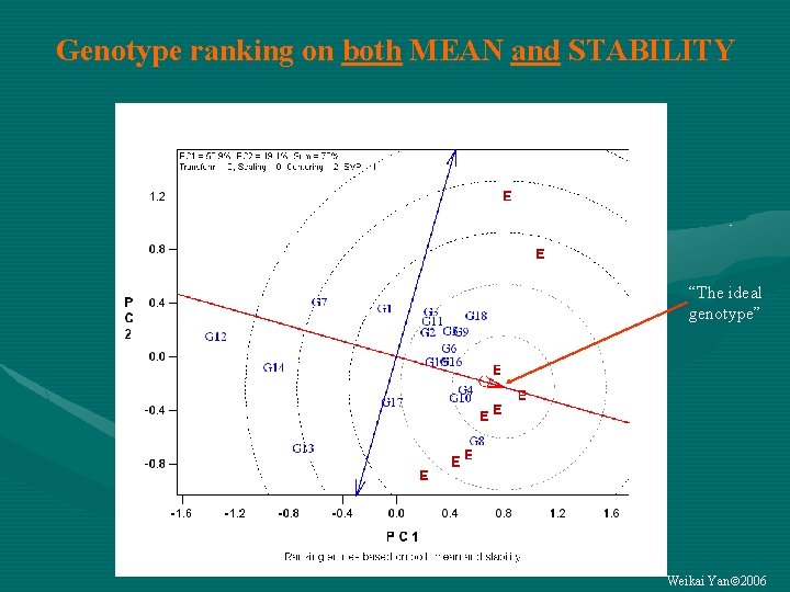
Genotype ranking on both MEAN and STABILITY “The ideal genotype” Weikai Yan 2006

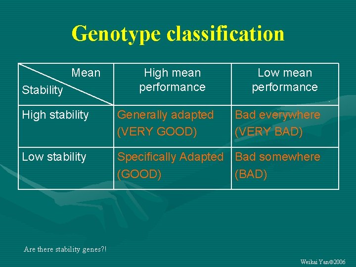
Genotype classification Mean Stability High mean performance Low mean performance High stability Generally adapted (VERY GOOD) Bad everywhere (VERY BAD) Low stability Specifically Adapted Bad somewhere (GOOD) (BAD) Are there stability genes? ! Weikai Yan 2006

G x E data analysis summary • 1) Mega-environment analysis • 2) Test environment evaluation • 3) Genotype evaluation Important comments: – (2) and (3) are meaningful only for a single mega-environment – Any stability analysis is meaningful only for a single megaenvironment – Any stability index can be used only as a modifier to the ranking based on mean performance Weikai Yan 2006

Other ways to view a GGE biplot Contact: wyan@ggebiplot. com

Inner-product property Weikai Yan 2006

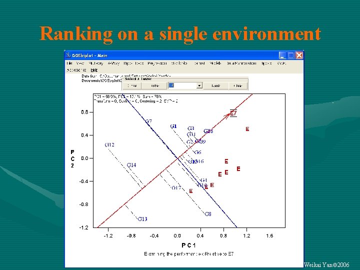
Ranking on a single environment Weikai Yan 2006

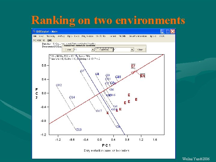
Ranking on two environments Weikai Yan 2006

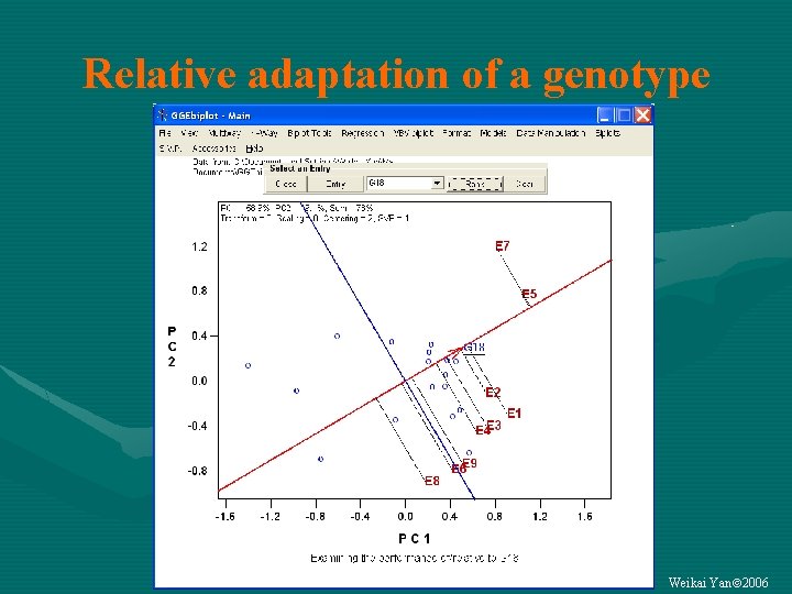
Relative adaptation of a genotype Weikai Yan 2006

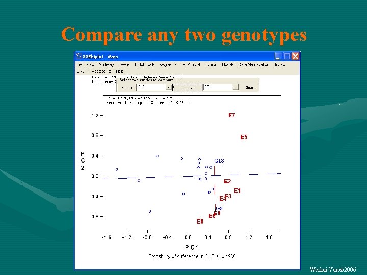
Compare any two genotypes Weikai Yan 2006

Biplot analysis of Genotype by trait data Contact: wyan@ggebiplot. com

Objectives of G By T data analysis • Genotype evaluation based on trait profiles • Relationship among breeding objectives Weikai Yan 2006

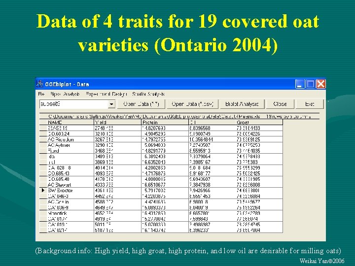
Data of 4 traits for 19 covered oat varieties (Ontario 2004) (Background info: High yield, high groat, high protein, and low oil are desirable for milling oats) Weikai Yan 2006

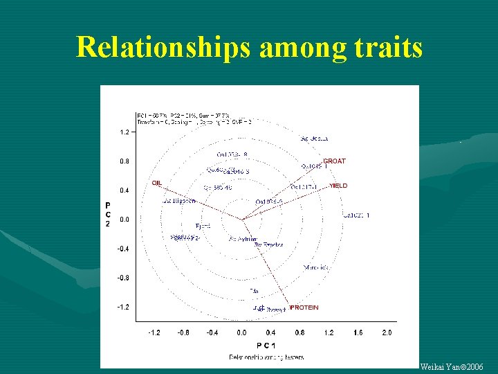
Relationships among traits Weikai Yan 2006

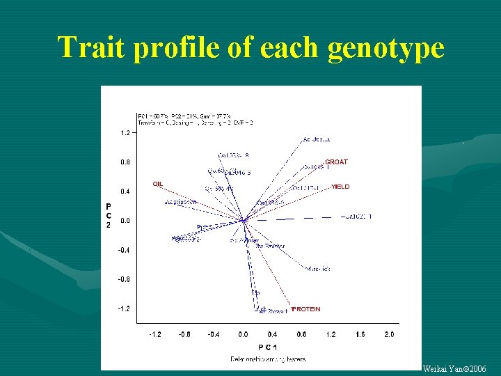
Trait profile of each genotype Weikai Yan 2006

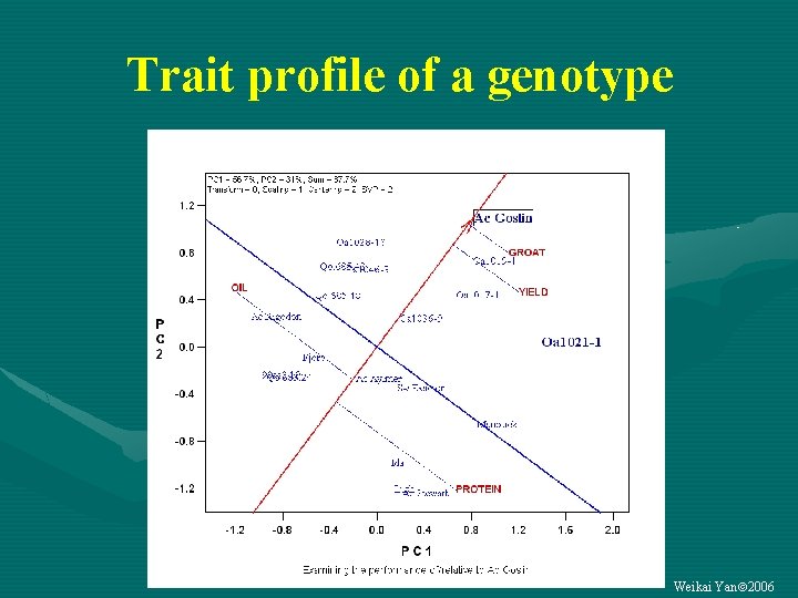
Trait profile of a genotype Weikai Yan 2006

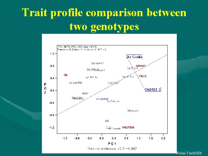
Trait profile comparison between two genotypes Weikai Yan 2006

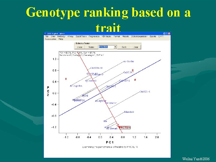
Genotype ranking based on a trait Weikai Yan 2006

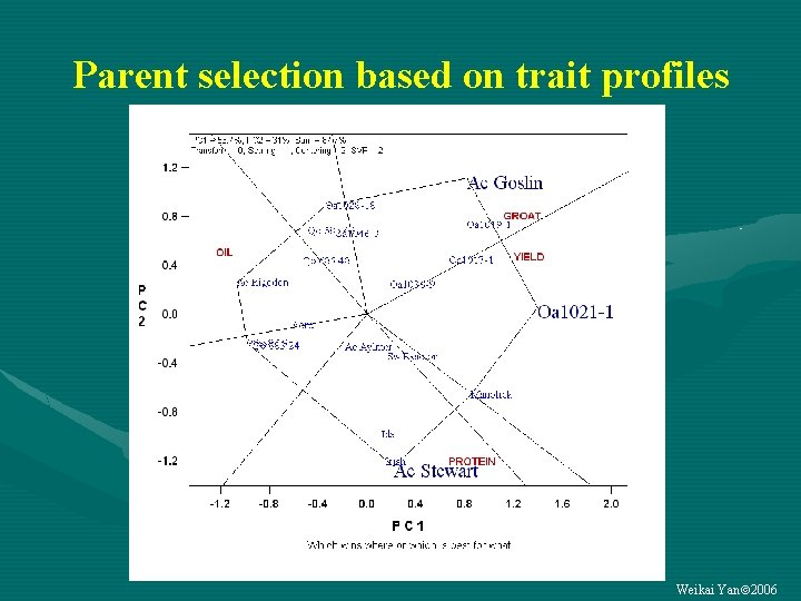
Parent selection based on trait profiles Weikai Yan 2006

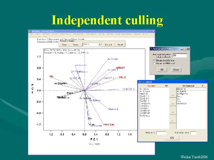
Independent culling Weikai Yan 2006

Fuller understanding of MET data are more informative than you thought Contact: wyan@ggebiplot. com

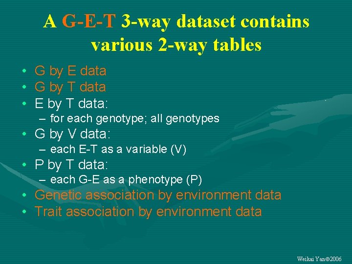
A G-E-T 3 -way dataset contains various 2 -way tables • G by E data • G by T data • E by T data: – for each genotype; all genotypes • G by V data: – each E-T as a variable (V) • P by T data: – each G-E as a phenotype (P) • Genetic association by environment data • Trait association by environment data Weikai Yan 2006

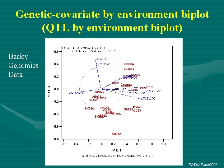
Genetic-covariate by environment biplot (QTL by environment biplot) Barley Genomics Data Weikai Yan 2006

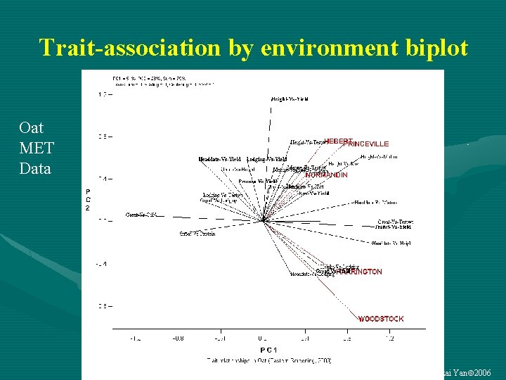
Trait-association by environment biplot Oat MET Data Weikai Yan 2006

Four-way data analysis • Year… Weikai Yan 2006

Conclusions Contact: wyan@ggebiplot. com

Conclusion (1) • “GGE biplot analysis” is an effective tool for G by E data analysis to achieve understandings about…. 1. 2. 3. 4. the target environment, the test environments, and the genotypes stability analysis is useful only to a single mega-environment Weikai Yan 2006

Conclusion (2) • “GGE biplot analysis” is an effective tool for G by T data analysis to achieve understandings about…. 1. the interconnected plant system, 2. positively correlated traits 3. negatively correlated traits 4. the strength and weakness of the genotypes Weikai Yan 2006

Conclusion (3) • “Biplot analysis” is an effective tool for other two-way table analysis – Marker by environment – QTL by environment – Gene by treatment – Diallel cross –… Weikai Yan 2006

Conclusion (4) • Biplot analysis can be VERY EASY… – From reading data to displaying the biplot: 2 seconds – Displaying any of the perspectives of a biplot and changing from one to another: 1 second – Displaying the biplot for any subset: 1 second – Learning how to use the software and interpret biplots: 30 minutes – Everything can be just one mouse-click away Weikai Yan 2006

Thank you Contact: Weikai Yan: wyan@ggebiplot. com web: www. ggebiplot. com Contact: wyan@ggebiplot. com