
BIOSTATISTICS Dr Atef A Masad Ph D Biomedicine
BIOSTATISTICS Dr Atef A Masad Ph. D Biomedicine Dr Atef A Masad Copyright © 2004 Pearson Education, Inc. , publishing as Benjamin Cummings 1
Some Basic Concepts The Meaning of Statistics “Statistics is the study of the methods and procedures for collecting, classifying, summarizing, and analyzing data and for making scientific conclusions from such data. ” Data - Data are the raw materials of statistics. - Data are the numerical information (numbers) that has been obtained on a set of objects and we use to interpret reality. Objects can be anything…e. g. , people, animals Example: The number of traffic accidents at certain junctions, the size of employments, or the number of patients visiting a clinic Dr Atef A Masad Copyright © 2004 Pearson Education, Inc. , publishing as Benjamin Cummings 2
Statistics is also used to indicate characteristics calculated for a set of data-for example, mean, standard deviation. Biostatistics: When the data being analyzed are derived from the biological sciences and medicine, we use the term biostatistics to distinguish this particular application of statistical tools and concepts. Dr Atef A Masad Copyright © 2004 Pearson Education, Inc. , publishing as Benjamin Cummings 3
Why Study Statistics? • A knowledge of statistics is essential for people going into research management or graduate study in a specialized area. • Researchers use statistical methods to quantify uncertainty in the outcomes, summarize and make sense of data, and compare the effectiveness of different treatments. • Federal government agencies and private • Companies rely heavily on statisticians’ input. • Important to review and understand the writings in scientific journals, which use statistical terminology and methodology. Dr Atef A Masad Copyright © 2004 Pearson Education, Inc. , publishing as Benjamin Cummings 4
• An understanding of statistics can help anyone discriminate between fact and fancy in everyday life-in reading newspapers and watching television, and in making daily comparisons and evaluations. • Finally, a course in statistics should help one know when, and for what purpose a statistician should be consulted. Dr Atef A Masad Copyright © 2004 Pearson Education, Inc. , publishing as Benjamin Cummings 5
Branches of Statistics • There are two major categories of statistics: • Descriptive and Inferential statistics. 1 Descriptive statistics ﺍﻹﺣﺼﺎﺀ ﺍﻟﻮﺻﻔﻲ • Comprise those methods concerned with collecting organizing, picturing, summarizing and describing a set of data so as to yield meaningful information. • Descriptive statistics provides information only about the collected data. • The construction of tables, charts, graphs, falls in the area categorized as descriptive statistics. Dr Atef A Masad Copyright © 2004 Pearson Education, Inc. , publishing as Benjamin Cummings 6
• An example of descriptive statistics is the decennial survey in some countries, in which all residents are requested to provide such information as age, sex, race, and marital status. • Example: presenting students marks in graphs or tables • The data obtained in such survey can then be compiled and arranged into tables and graphs that describe the characteristics of the population at a given time. Dr Atef A Masad Copyright © 2004 Pearson Education, Inc. , publishing as Benjamin Cummings 7
• 2 Inferential statistics ( ﺍﻹﺳﺘﺪﻻﻟﻲ )ﺍﻹﺣﺼﺎﺀ ﺍﻹﺳﺘﻨﺘﺎﺟﻲ • Comprise those methods concerned with the analysis of information from a sample or a subset of data to draw conclusions regarding the population or the entire set of data. • An example is an opinion survey, such as the pre-election Poll, which attempts to draw inferences as to the outcome of an election. • In such survey, a sample of individuals (frequently fewer than 2000) is selected; their preferences are tabulated, and inferences are made as to how millions of persons would vote if an election were held that day. Dr Atef A Masad Copyright © 2004 Pearson Education, Inc. , publishing as Benjamin Cummings 8
Sources of Data 1. Routinely kept records: Hospital medical records, for example, contain immense amounts of information on patients. 2. Surveys: Data is gathered by asking people questions. Followed when the data needed are not available from routinely kept records. • For example, if the admission forms do not contain a question on mode of transportation, we may conduct a survey among patients to obtain this information. • The study of the psychological effects of explosion of the atomic bomb on the inhabitants of Hiroshima and Nagasaki is another example of a survey. Dr Atef A Masad Copyright © 2004 Pearson Education, Inc. , publishing as Benjamin Cummings 9
Methods of survey: • Personal interview • Telephone interview • Questionnaires 3. Experiments: for example, the effect of specific medication on specific disease. 4. Observations attained by naked eyes or through video camera, ……. . etc. 5. External sources: e. g. published reports, commercially available data banks, or the research literature. Dr Atef A Masad Copyright © 2004 Pearson Education, Inc. , publishing as Benjamin Cummings 10
• Variables • The variable is the characteristic of the people or object included in a study to be measured or observed. Examples include: Age, weight, height, marital status, or blood group • 2 Types of Variables • Qualitative (independent) variables ﻣﺘﻐﻴﺮﻣﺴﺘﻘﻞ ﻭﺛﺎﺑﺖ • Variables that yield observations on which individuals can be categorized according to some characteristic, examples include; occupation, sex, marital status, and education level. • Quantitative (dependent) variables ﻣﺘﻐﻴﺮ ﺗﺎﺑﻊ ﻭﻣﺘﻐﻴﺮ • Variables that yield observations that can be counted or measured, example include; weight, height, and serum cholesterol. Dr Atef A Masad Copyright © 2004 Pearson Education, Inc. , publishing as Benjamin Cummings 11
Quantitative variables can be further classified as discrete or continuous. ●Discrete variables ﺍﻟﻤﺘﻐﻴﺮ ﺍﻟﻤﻨﻔﺼﻞ ● ﻳﺄﺨﺬ ﻗﻴﻤﺎ ﻗﺎﺑﻠﻪ ﻟﻠﻌﺪ ●A variable is called discrete if it has only a countable number of values. Usually these will be whole numbers (integers) such as 3, 5, 9, and 23 and none in between (i. e. they usually don’t have decimal values). ●For example, the number of patients in a hospital may be 178 or 179, but it cannot be any value between these two. ●The number of syringes used in a clinic on any given day. ●The number of children in one family ●The number of times that you visited a doctor. ●The number of missing teeth Dr Atef A Masad 12 Copyright © 2004 Pearson Education, Inc. , publishing as Benjamin Cummings
�� Continuous ﺍﻟﻤﺘﻐﻴﺮ ﺍﻟﻤﺘﺼﻞ ﻳﻜﻮﻥ ﺗﺄﺜﻴﺮﻩ ﻋﻠﻰ ﻓﺘﺮﺍﺕ ﻣﺘﻮﺍﺻﻠﻪ • ex. Temperature can be increased or decreased gradually not suddenly). They are measured on some scale in terms of some measurement unit such as kilograms, meters, mmol/l, degree Centigrade, weight, height, length…. . etc. • Example: a researcher can study the effect of sex (independent variable) or income (continuous variable) on education progress(Qualitative (dependent) variable). Dr Atef A Masad Copyright © 2004 Pearson Education, Inc. , publishing as Benjamin Cummings 13
• Scale (or Level) of Measurements ( )ﻣﺴﺘﻮﻳﺎﺕ ﺍﻟﻘﻴﺎﺱ • Giving a numerical value for observations or things seen • There are four levels of measurement or scales of measurements into which data can be classified. • • These are: nominal ﺇﺳﻤﻲ , ordinal ﺗﺮﺗﻴﺒ , interval ﺍﻟﻤﺴﺎﻓﻲ , or ratio ﺍﻟﻤﺴﺎﻓﻲ. Dr Atef A Masad Copyright © 2004 Pearson Education, Inc. , publishing as Benjamin Cummings 14
1 • Nominal ﺇﺳﻤﻲ ﻳﺴﺘﺨﺪﻡ ﻟﺘﺤﺪﻳﺪ ﻫﻮﻳﺔ ﺍﻻﻓﺮﺍﺩ ﺍﻭ ﺍﻟﻌﻨﺎﺻﺮ • The lowest level of the measurement scale types is the nominal scale. Nominal scale data are divided into qualitative categories or groups, such as male/female, black/white, well/sick, child/adult, and married/ not married. • Numbers, when used, are used as labels only and have no numerical meaning such as telephone or car numbers. Nominal scale data cannot be arranged in an ordering scheme. • Arithmetic operations of addition, subtraction, multiplication, and division are not performed for nominal data. Example: Gender Data • Dr. Male, Female Atef A Masad 15 Copyright © 2004 Pearson Education, Inc. , publishing as Benjamin Cummings
2 • Ordinal ﺗﺮﺗﻴﺒ - ﻣﻘﻴﺎﺱ ﺍﻟﺮﺗﺒﻪ ﻭﺍﻟﺘﺮﺗﻴﺐ • Data at the ordinal level may be arranged in some order, but actual differences between data values either cannot be determined or are meaningless. • For example, class may be ranked 1 st/2 nd/3 rd. • There is no information about the size of the interval • no conclusion can be drawn about whether the difference between the first and second student is the same as the difference between the second and third. • More examples include, the degree of pain (severe, moderate, mild, none), the age group (baby, infant, child, adult, geriatric). Dr Atef A Masad Copyright © 2004 Pearson Education, Inc. , publishing as Benjamin Cummings 16
3. Interval ﻣﻘﻴﺎﺱ ﺍﻟﻤﺴﺎﻓﺔ For example, on the Celsius scale the difference between 100 and 90°C is the same as the difference between 50°C and 40°C. • However because interval scales do not have an absolute zero, ratios of scores are not meaningful: it is not correct to say 20 °C is twice as hot as 10 °C or 100°C is not twice as hot as 50°C, because 0°C does not represent the point at which there is no heat, but the freezing point of water. • Calendar times are also interval measurements, since the date 0 A. D. does not signify “no time”. Dr Atef A Masad Copyright © 2004 Pearson Education, Inc. , publishing as Benjamin Cummings 17
• Also, An IQ “Intelligent Quotient” of zero would not mean no intelligence at all, but serious thinker or problem in using materials of the test. • Interval-level data have no absolute zero point or starting point. Consequently, differences are meaningful but ratios of data are not. Dr Atef A Masad Copyright © 2004 Pearson Education, Inc. , publishing as Benjamin Cummings 18
• Ratio ﺍﻟﻨﺴﺒﻲ • A ratio scale has the same properties as an interval scale; but because it has an absolute zero, meaningful ratios do exist. • Most biomedical variables form a ratio scale: weight in grams or pounds, time in seconds or days, blood pressure in millimeters of mercury and pulse rate are all ratio scale data. • The only ratio scale of a zero pulse rate indicates an absolute lake of heartbeat. • Therefore, it is correct to say that a pulse rate of 120 is twice as fast as a pulse rate of 60. More examples include; height, heart beat, …………. . etc Dr Atef A Masad Copyright © 2004 Pearson Education, Inc. , publishing as Benjamin Cummings 19
2 Populations and Samples ( ( ﺍﻟﻤﺠﺘﻤﻌﺎﺕ ﻭ ﺍﻟﻌﻴﻨﺎﺕ • The term population refers to a collection of people or objects that share common observable characteristics. • For example, a population could be all of the people who live in your city, all of the students enrolled in a particular university, or all of the people who are troubled by a certain disease (e. g. , all women diagnosed with breast cancer during the last five years). • Generally, researchers are interested in particular characteristics of a population, not the characteristics that define the population but rather such features as • height, weight, gender, age, heart rate, and systolic or diastolic blood pressure. Copyright © 2004 Pearson Education, Inc. , publishing as Benjamin Cummings
A sample is a subset of data selected from a population. The number of elements in the sample is called the sample size. The primary objective for selecting a sample from a population is to draw inference (conclusion) about that population. Parameters and statistics • A parameter is a characteristic of or a fact about a population. • A statistic is a characteristic of or a fact about a sample. Sampling Procedure by which some members of a given population are selected as representatives of the entire population Dr Atef A Masad Copyright © 2004 Pearson Education, Inc. , publishing as Benjamin Cummings 21
Why do we sample? Why not study the entire population? • There are many reasons to study samples instead of populations: • A study of an entire population is impossible in most situations because the population may be hypothetical (e. g. patients who may receive a treatment in the future). • less expensive than studying an entire population. • It is labour-intensive to study the entire population • more quickly than populations. • Some testing is inherently destructive: We can't drain all the blood from a person and count every white cell. Copyright © 2004 Pearson Education, Inc. , publishing as Benjamin Cummings
How Samples Are Selected? • Simple random samples ﺍﻟﻌﻴﻨﺔ ﺍﻟﻌﺸﻮﺍﺋﻴﺔ ﺍﻟﺒﺴﻴﻄﺔ • It is a sample drawn so that every • element in the population has an equal probability of being included. • There are two ways for selecting simple random sample • 1. Lottery method • Procedure • - Number all units • - Randomly draw units • Example: evaluate the prevalence of tooth decay among the 800 children attending a school Copyright © 2004 Pearson Education, Inc. , publishing as Benjamin Cummings
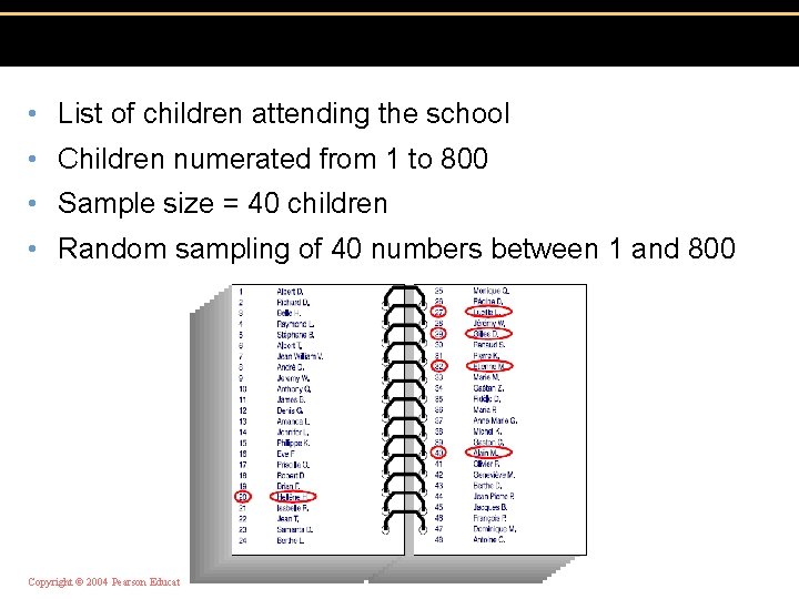
• List of children attending the school • Children numerated from 1 to 800 • Sample size = 40 children • Random sampling of 40 numbers between 1 and 800 Copyright © 2004 Pearson Education, Inc. , publishing as Benjamin Cummings
2. Random number table (described at the end) Systematic sampling ﻃﺮﻳﻘﺔ ﺍﻟﻌﻴﻨﺔ ﺍﻟﻤﻨﺘﻈﻤﺔ We randomly select a first case and then proceed by selecting every nth case. Where n is determined by dividing the number of items in the sampling frame (a complete list of people or objects constituting the population) by the desired sample size. Copyright © 2004 Pearson Education, Inc. , publishing as Benjamin Cummings
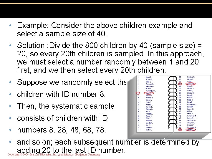
• Example: Consider the above children example and select a sample size of 40. • Solution : Divide the 800 children by 40 (sample size) = 20, so every 20 th children is sampled. In this approach, we must select a number randomly between 1 and 20 first, and we then select every 20 th children. • Suppose we randomly select the • children with ID number 8. • Then, the systematic sample • consists of children with ID • numbers 8, 28, 48, 68, 78, • and so on; each subsequent number is determined by adding 20 to the last ID number. Copyright © 2004 Pearson Education, Inc. , publishing as Benjamin Cummings
• Stratified Sampling ﻃﺮﻳﻘﺔ ﺍﻟﻌﻴﻨﻪ ﺍﻟﻄﺒﻘﻴﺔ • Strata are groups or classes inside a population that share a common characteristic. • Procedure for selecting of stratified sampling • The population is first divided into at least two distinct strata or groups. • Then a simple random sample of a certain size is drawn from each stratum. • The groups or strata are often sampled in proportion to their actual percentage of occurrence in the overall population. • Combine results of all strata. Copyright © 2004 Pearson Education, Inc. , publishing as Benjamin Cummings
• This stratification results in greater representativeness. For example, instead of • drawing one sample of 10 people from a total population consisting of 500 black and 500 white people, two random samples of five could be taken from each racial group (or stratum) separately, thus guaranteeing the racial representativeness of the resulting overall sample of 10. • Other strata might be men or women, department, location, age, field of study and so on. Copyright © 2004 Pearson Education, Inc. , publishing as Benjamin Cummings
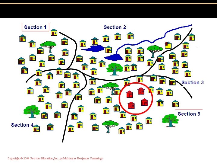
• Cluster Sampling ﻃﺮﻳﻘﺔ ﺍﻟﻌﻴﻨﻪ ﺍﻟﻌﻨﻘﻮﺩﻳﺔ • In cluster sampling we begin by dividing the demographic area into sections. • Then we randomly select sections or clusters. • Every member of the cluster is included in the sample. For example, in conducting a survey of school children in a large city, we could first randomly select 4 schools • and then include all the children from each selected school. • This technique is more economical than the random selection of persons throughout the city. Copyright © 2004 Pearson Education, Inc. , publishing as Benjamin Cummings
Copyright © 2004 Pearson Education, Inc. , publishing as Benjamin Cummings
Convenience Sampling ( ( ﺍﻟﻌﻴﻨﺔ ﺍﻟﻤﻴﺴﺮﺓ • Convenience sampling is just what the name suggests: the patients or samples are selected by a random method that is easy to carry out. • Some researchers refer to these types of samples as “grab bag” samples. • Ex: MOH evaluation • Example, when studying patients with a particular clinical condition, • we may choose a single hospital, and investigate some or all of the patients with the condition in that hospital. • Which is not representative to the whole population • Convenience sampling is very easy to do, but it's probably the worst technique to use. Copyright © 2004 Pearson Education, Inc. , publishing as Benjamin Cummings
• For example suppose a catheter ablation treatment is known to have a 95% chance of success. • That means that we expect only about one failure in a sample of size 20. • However, even though the probability is very small, it is possible that we could select a random sample of 20 individuals with the outcome that all 20 individuals have failed ablation procedures. • Results of studies based on convenience samples are descriptive and may be used to suggest future research, but they should not be used to draw inferences about the population under study. Dr Atef A Masad Copyright © 2004 Pearson Education, Inc. , publishing as Benjamin Cummings 32
• Judgment Sampling ( ( ﺍﻟﻌﻴﻨﺔ ﺍﻟﻬﺎﺩﻓﺔ • The person most knowledgeable on the subject of the study selects elements of the population that he or she feels are most representative of the population. • Example: A reporter might sample three or four ministers, judging them as reflecting the • general opinion of the government. Copyright © 2004 Pearson Education, Inc. , publishing as Benjamin Cummings
• How to select a Random Sample? • One of the easiest ways to select a random sample is to use a random number table. • Such tables are easy to find; they are in many statistical texts and mathematical handbooks. • Many calculators and computers also generate random numbers. • A portion of a random number table is reproduced in Table 2. 1. • Random number tables are prepared in such a way that each digit gets equal representation. Copyright © 2004 Pearson Education, Inc. , publishing as Benjamin Cummings
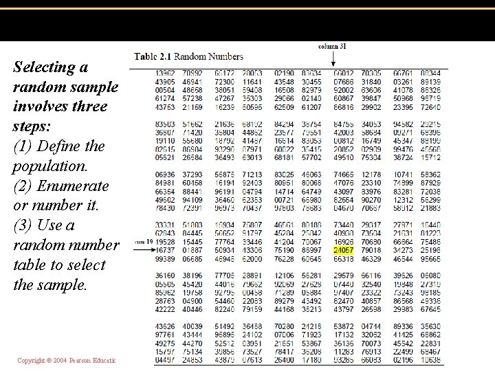
Selecting a random sample involves three steps: (1) Define the population. (2) Enumerate or number it. (3) Use a random number table to select the sample. Copyright © 2004 Pearson Education, Inc. , publishing as Benjamin Cummings
• Example: • Select 10 persons from a population of 83 cases in a hypertension (high blood pressure) study (see Table 2. 2). • Solution: • Observe that the population is clearly defined: 83 cases classified according to their diastolic blood pressure, sex, and dietary status. • Also note that the cases have been numbered arbitrarily from 1 to 83. Copyright © 2004 Pearson Education, Inc. , publishing as Benjamin Cummings
• If the random number table covered four pages, you might flip a coin twice and arbitrarily agree to assign HH (two heads) to page 1, HT to page 2, TH to page 3, and TT to page 4. • Suppose you flip heads on both tosses (HH); you then turn to page 1. • To choose an arbitrary starting place, you could blindly stab at row 19 and column 31. (This procedure is illustrated in Table 2. 1. ) The row-column • intersection of the starting place should be recorded, just in case you wish later to verify • your selection and hence your sample. • Next, read the two-digit numeral that falls at that spot. Copyright © 2004 Pearson Education, Inc. , publishing as Benjamin Cummings
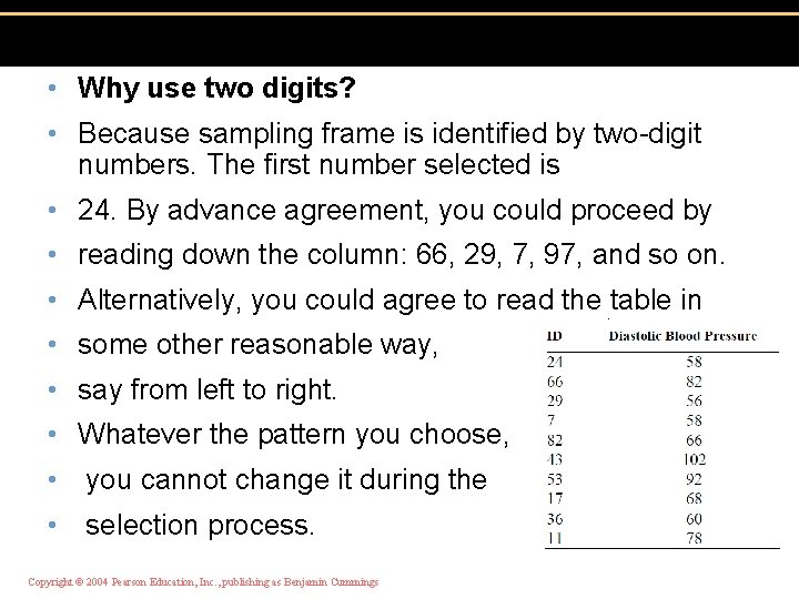
• Why use two digits? • Because sampling frame is identified by two-digit numbers. The first number selected is • 24. By advance agreement, you could proceed by • reading down the column: 66, 29, 7, 97, and so on. • Alternatively, you could agree to read the table in • some other reasonable way, • say from left to right. • Whatever the pattern you choose, • you cannot change it during the • selection process. Copyright © 2004 Pearson Education, Inc. , publishing as Benjamin Cummings
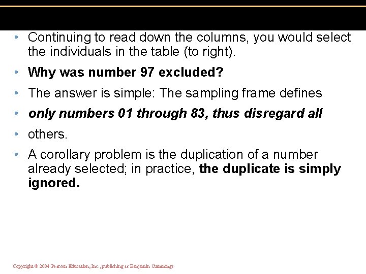
• Continuing to read down the columns, you would select the individuals in the table (to right). • Why was number 97 excluded? • The answer is simple: The sampling frame defines • only numbers 01 through 83, thus disregard all • others. • A corollary problem is the duplication of a number already selected; in practice, the duplicate is simply ignored. Copyright © 2004 Pearson Education, Inc. , publishing as Benjamin Cummings
• Simple random sampling is one of the statistician's most vital tools and is used in countless applications. • It is the basic building block for every method of sampling, no matter how sophisticated. • Occasionally however, it may be uneconomical or impractical to implement a random selection scheme that requires details of the entire population. Dr Atef A Masad Copyright © 2004 Pearson Education, Inc. , publishing as Benjamin Cummings 40
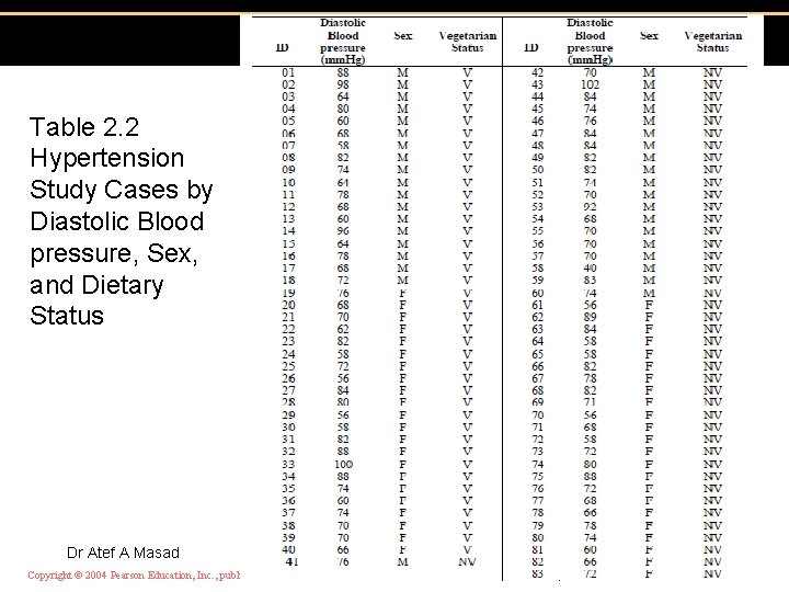
Table 2. 2 Hypertension Study Cases by Diastolic Blood pressure, Sex, and Dietary Status Dr Atef A Masad Copyright © 2004 Pearson Education, Inc. , publishing as Benjamin Cummings 41
3 Organizing and Displaying Data • Any survey or experiment yields a list of observations. • These need to be organized and summarized in a logical fashion so that we may perceive the outcome clearly. • Tables and graphs are popularly used to organize and summarize data and description of data. Dr Atef A Masad Copyright © 2004 Pearson Education, Inc. , publishing as Benjamin Cummings 42
A. Frequency Tables/ Frequency Distributions • Considerable information can be obtained from large masses of statistical data by grouping the raw data into classes and determining the number of observations that fall in each of the classes. • Such an arrangement is called a frequency distribution or frequency table ���������. • Frequency table may be the most convenient way of summarizing or displaying data. • The types of frequency distributions that will be considered here are categorical or qualitative frequency distributions, and grouped frequency distributions. Dr Atef A Masad Copyright © 2004 Pearson Education, Inc. , publishing as Benjamin Cummings 43
• Categorical frequency distributions • represent data that can be placed in specific categories, such as gender, hair color, or blood group. • Example: The blood types of 25 blood donors are given below. Summarize the data • using a frequency distribution. Dr Atef A Masad Copyright © 2004 Pearson Education, Inc. , publishing as Benjamin Cummings 44
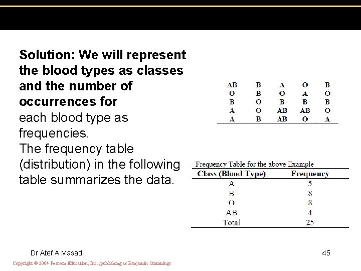
Solution: We will represent the blood types as classes and the number of occurrences for each blood type as frequencies. The frequency table (distribution) in the following table summarizes the data. Dr Atef A Masad Copyright © 2004 Pearson Education, Inc. , publishing as Benjamin Cummings 45
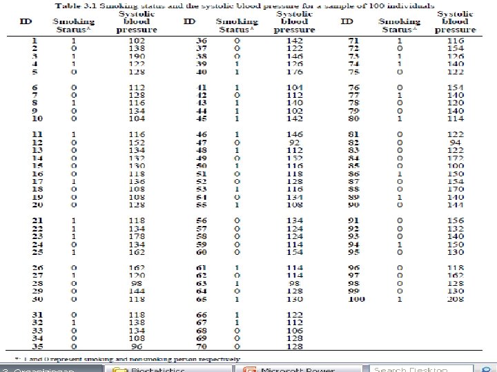
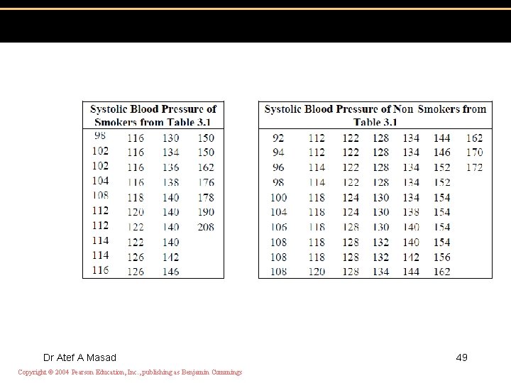
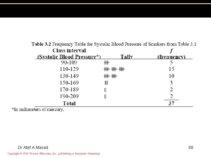
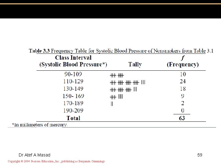
• Grouped Frequency Distributions • A grouped frequency distribution is obtained by constructing class intervals ﻓﺌﺎﺕ for the data, and then listing the corresponding number of values (frequency count) in each interval. • Tables 3. 2 and 3. 3 are examples of frequency tables, constructed from the systolic blood pressure readings (by smoking status) of Table 3. 1. Dr Atef A Masad Copyright © 2004 Pearson Education, Inc. , publishing as Benjamin Cummings 46
Dr Atef A Masad Copyright © 2004 Pearson Education, Inc. , publishing as Benjamin Cummings 47
• How to construct a frequency table? • 1. Arrange the data into an array, a listing of all observations from smallest to largest in order to determine the interval ﺍﻟﻔﺌﻪ spanned by the data. • We find that the blood pressure interval for smokers for example is 98 -208. Dr Atef A Masad Copyright © 2004 Pearson Education, Inc. , publishing as Benjamin Cummings 48
Dr Atef A Masad Copyright © 2004 Pearson Education, Inc. , publishing as Benjamin Cummings 49
• 2. Determine the range (ﺍﻟﻤﺪﻯ R) from the difference between the smallest and largest value in the set of observations i. e. R = largest data value – smallest data value • = 208 -98 =110 mm. • 3. Divide the range into a number of equal and non overlapping segments called class intervals ﻃﻮﻝ ﺍﻟﻔﺌﻪ. • Important Note • The number of intervals in general should range from 5 to 15. Dr Atef A Masad Copyright © 2004 Pearson Education, Inc. , publishing as Benjamin Cummings 50
• With too many class intervals , the data are not summarized enough for a clear visualization of how they are distributed. • With too few, the data are over-summarized and some of the details of the distribution may lost Dr Atef A Masad Copyright © 2004 Pearson Education, Inc. , publishing as Benjamin Cummings 51
• Sturges’s formula and the desired number of class intervals • Those who wish more specific guidance in the matter of deciding how many class intervals are needed may use Sturges’s formula; • k = 1 + 3. 322(log 10 n), • where k stands for the number of class intervals and n is the number of values in the data • set under consideration (or the sample size) Dr Atef A Masad Copyright © 2004 Pearson Education, Inc. , publishing as Benjamin Cummings 52
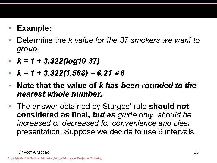
• Example: • Determine the k value for the 37 smokers we want to group. • k = 1 + 3. 322(log 10 37) • k = 1 + 3. 322(1. 568) = 6. 21 ≅ 6 • Note that the value of k has been rounded to the nearest whole number. • The answer obtained by Sturges’ rule should not considered as final, but as guide only, should be increased or decreased for convenience and clear presentation. Suppose we decide to use 6 intervals. Dr Atef A Masad Copyright © 2004 Pearson Education, Inc. , publishing as Benjamin Cummings 53
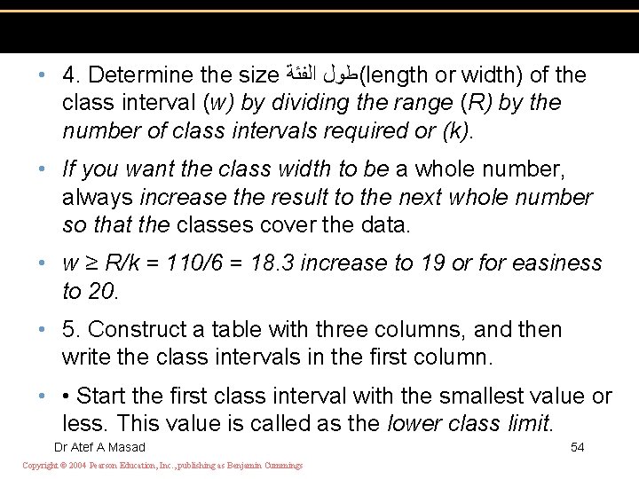
• 4. Determine the size (ﻃﻮﻝ ﺍﻟﻔﺌﺔ length or width) of the class interval (w) by dividing the range (R) by the number of class intervals required or (k). • If you want the class width to be a whole number, always increase the result to the next whole number so that the classes cover the data. • w ≥ R/k = 110/6 = 18. 3 increase to 19 or for easiness to 20. • 5. Construct a table with three columns, and then write the class intervals in the first column. • • Start the first class interval with the smallest value or less. This value is called as the lower class limit. Dr Atef A Masad Copyright © 2004 Pearson Education, Inc. , publishing as Benjamin Cummings 54
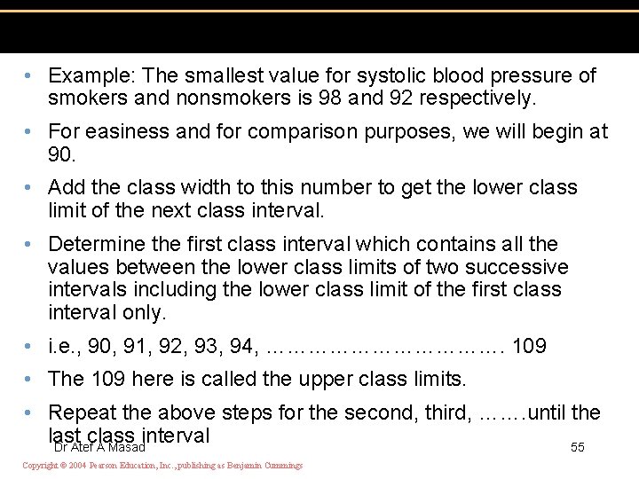
• Example: The smallest value for systolic blood pressure of smokers and nonsmokers is 98 and 92 respectively. • For easiness and for comparison purposes, we will begin at 90. • Add the class width to this number to get the lower class limit of the next class interval. • Determine the first class interval which contains all the values between the lower class limits of two successive intervals including the lower class limit of the first class interval only. • i. e. , 90, 91, 92, 93, 94, ………………. 109 • The 109 here is called the upper class limits. • Repeat the above steps for the second, third, ……. until the last class interval Dr Atef A Masad 55 Copyright © 2004 Pearson Education, Inc. , publishing as Benjamin Cummings
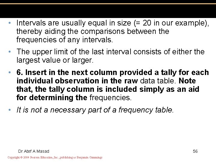
• Intervals are usually equal in size (= 20 in our example), thereby aiding the comparisons between the frequencies of any intervals. • The upper limit of the last interval consists of either the largest value or larger. • 6. Insert in the next column provided a tally for each individual observation in the raw data table. Note that, the tally column is included simply as an aid for determining the frequencies. • It is not a necessary part of a frequency table. Dr Atef A Masad Copyright © 2004 Pearson Education, Inc. , publishing as Benjamin Cummings 56
• 7. Sum the tally in each row and record them in the third column entitled Frequency (f). • 8. Sum the frequency column (n). This serves as a useful check that all data have been included in the table. • Note • Frequency tables should be numbered, includes an appropriate descriptive title, specify the units of measurement, and cite the source of data. Dr Atef A Masad Copyright © 2004 Pearson Education, Inc. , publishing as Benjamin Cummings 57
Dr Atef A Masad Copyright © 2004 Pearson Education, Inc. , publishing as Benjamin Cummings 58
Dr Atef A Masad Copyright © 2004 Pearson Education, Inc. , publishing as Benjamin Cummings 59
• Frequency Tables with class boundaries • Class boundaries may be used in place of class limits. Class boundaries are points that separate the true upper limit of one class and the true lower limit of the next. • Class boundaries ﺣﺪﻭﺩ ﺍﻟﻔﺌﺎﺕ can be easily obtained by applying the formula: • Upper limit of one Class boundary = upper limit of one class + lower limit of next class/2 Dr Atef A Masad Copyright © 2004 Pearson Education, Inc. , publishing as Benjamin Cummings 60
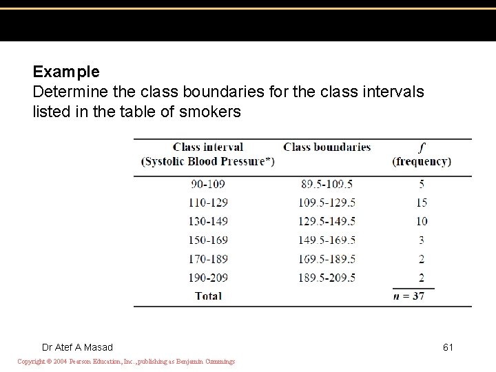
Example Determine the class boundaries for the class intervals listed in the table of smokers Dr Atef A Masad Copyright © 2004 Pearson Education, Inc. , publishing as Benjamin Cummings 61
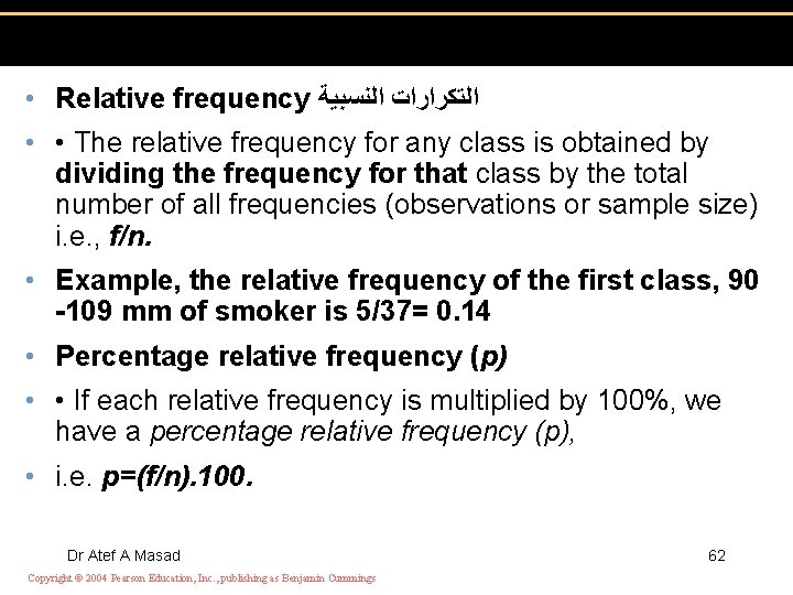
• Relative frequency ﺍﻟﺘﻜﺮﺍﺭﺍﺕ ﺍﻟﻨﺴﺒﻴﺔ • • The relative frequency for any class is obtained by dividing the frequency for that class by the total number of all frequencies (observations or sample size) i. e. , f/n. • Example, the relative frequency of the first class, 90 -109 mm of smoker is 5/37= 0. 14 • Percentage relative frequency (p) • • If each relative frequency is multiplied by 100%, we have a percentage relative frequency (p), • i. e. p=(f/n). 100. Dr Atef A Masad Copyright © 2004 Pearson Education, Inc. , publishing as Benjamin Cummings 62
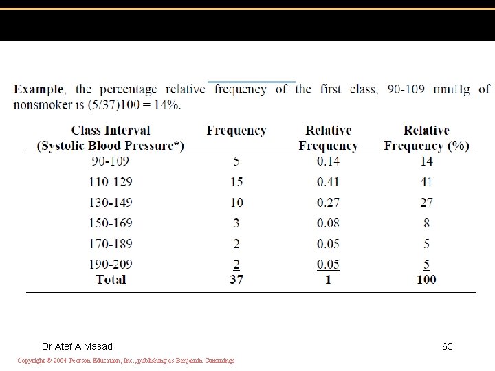
Dr Atef A Masad Copyright © 2004 Pearson Education, Inc. , publishing as Benjamin Cummings 63
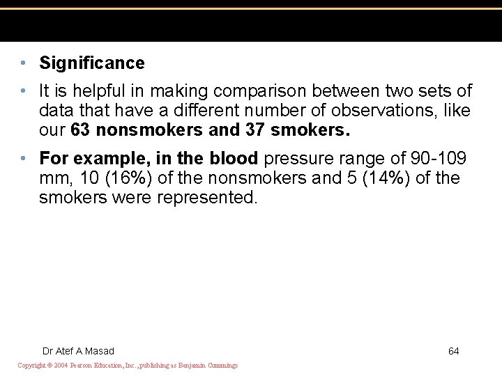
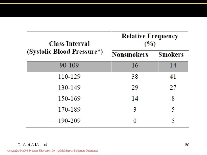
• Significance • It is helpful in making comparison between two sets of data that have a different number of observations, like our 63 nonsmokers and 37 smokers. • For example, in the blood pressure range of 90 -109 mm, 10 (16%) of the nonsmokers and 5 (14%) of the smokers were represented. Dr Atef A Masad Copyright © 2004 Pearson Education, Inc. , publishing as Benjamin Cummings 64
Dr Atef A Masad Copyright © 2004 Pearson Education, Inc. , publishing as Benjamin Cummings 65
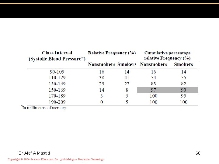
• Cumulative percentage relative frequency , ﺍﻟﺘﻜﺮﺍﺭ ﺍﻟﻨﺴﺒﻲ ﺍﻟﻤﺘﺠﻤﻊ • • It is also known as cumulative percentage • • It shows the percentage of elements lying within and below each class interval • • Cumulative percentage relative frequency can be computed by cumulating the percentage relative frequencies of each of the various class intervals. • For nonsmokers (Table 3. 4), the cumulative percentage for the first four intervals is • 16 + 38 + 29 + 14 = 97%. Dr Atef A Masad Copyright © 2004 Pearson Education, Inc. , publishing as Benjamin Cummings 66
• Significance: Make a rapid comparison of entire frequency distributions, ruling out any • need to compare individual class intervals. In our example, for example, 97% of the • nonsmokers in the sample have a systolic blood pressure below 169. 5. By comparison, • 90% of the smokers have a blood pressure below the same level. An alternate way of • looking at this is to note that 3% of the nonsmokers and 10% of the smokers have a • systolic blood pressure above 169. 5. Dr Atef A Masad Copyright © 2004 Pearson Education, Inc. , publishing as Benjamin Cummings 67
Dr Atef A Masad Copyright © 2004 Pearson Education, Inc. , publishing as Benjamin Cummings 68
• B. Graphing Representation of Data • The second way of displaying data is by use of graphs. Although such visual aids are • even easier to read than tables, they often do not give the same detail. • It is essential that each graph be self-explanatory that is, it should has • �� a descriptive title, • �� labeled axes, • �� An indication of the units of observation. • �� An effective graph should not attempt to present so much information that it is Dr Atef A Masad • difficult to comprehend. Copyright © 2004 Pearson Education, Inc. , publishing as Benjamin Cummings 69
• 1. Histograms ﺍﻟﻤﺪﺭﺝ ﺍﻟﺘﻜﺮﺍﺭﻱ • A histogram is a graphical display of a frequency distribution that uses classes and • vertical bars (rectangles) of various heights to represent the frequencies. Histograms are • useful when the data values are quantitative. A histogram gives an estimate of the shape • of the distribution of the population from which one sample was taken. Dr Atef A Masad 70 Copyright © 2004 Pearson Education, Inc. , publishing as Benjamin Cummings
• To make a histogram • • Make frequency table that shows class intervals and class frequencies. • • Determine the class boundaries for each class interval. • • Draw both abscissa (X or horizontal axis), which depicts the class boundaries (not • limits), and a perpendicular ordinate (Y or vertical axis), which depicts the • frequency (or relative frequency) of observations. • • Begin the vertical scale at zero. • • Dr Atef A Masad Copyright © 2004 Pearson Education, Inc. , publishing as Benjamin Cummings 71
• Once the scales have been laid out, a vertical bar is constructed above each class • interval equal in height to its class frequency. • • When the size of class intervals is equal, frequencies are represented by both • the height and the area of each bar. The total area represents 100%. Dr Atef A Masad Copyright © 2004 Pearson Education, Inc. , publishing as Benjamin Cummings 72
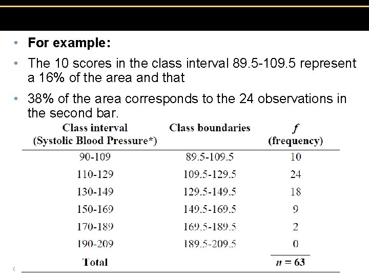
• For example: • The 10 scores in the class interval 89. 5 -109. 5 represent a 16% of the area and that • 38% of the area corresponds to the 24 observations in the second bar. Dr Atef A Masad Copyright © 2004 Pearson Education, Inc. , publishing as Benjamin Cummings 73
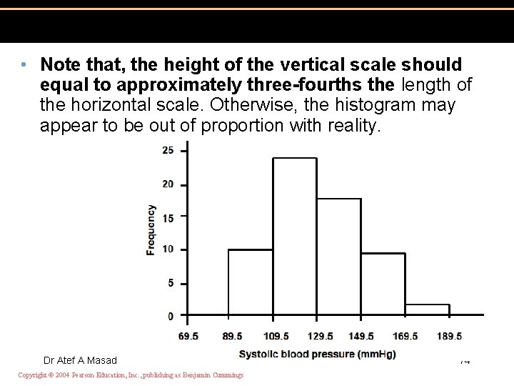
• Note that, the height of the vertical scale should equal to approximately three-fourths the length of the horizontal scale. Otherwise, the histogram may appear to be out of proportion with reality. Dr Atef A Masad Copyright © 2004 Pearson Education, Inc. , publishing as Benjamin Cummings 74
• 2. Frequency Polygons ﺍﻟﻤﻀﻠﻊ ﺍﻟﺘﻜﺮﺍﺭﻱ • A histogram gives the impression that frequencies jump suddenly from one class to the next. • If you want to emphasize the continuous rise or fall of the frequencies, you can use a frequency polygon or line graph. • Frequency polygon uses the same axes as the histogram. • It is constructed by marking a dot at the class midpoint of the class interval at the • height of the class frequency. • class midpoint = lower class boundary (limit) + upper Dr Atef A Masad 75 class boundary (limit) Copyright © 2004 Pearson Education, Inc. , publishing as Benjamin Cummings
Dr Atef A Masad Copyright © 2004 Pearson Education, Inc. , publishing as Benjamin Cummings 76
- Slides: 76