Biomedical Signal processing matlab Zhongguo Liu Biomedical Engineering

Biomedical Signal processing matlab 信号处理函数 Zhongguo Liu Biomedical Engineering School of Control Science and Engineering, Shandong University 2021/9/7 1 Zhongguo Liu_Biomedical Engineering_Shandong Univ.
 Signal Processing (信号处理 具箱) Wavelet (小波 具箱) Image Processing(图象处理 具箱)")
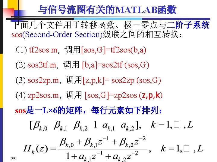
MATLAB与信号处理直接有关的 具箱 ( Toolbox) Signal Processing (信号处理 具箱) Wavelet (小波 具箱) Image Processing(图象处理 具箱) Higher-Order Spectral Analysis (高阶谱分析 具箱) 3
 (通信) System Identification (系统辨识) Statistics Neural Network 4")
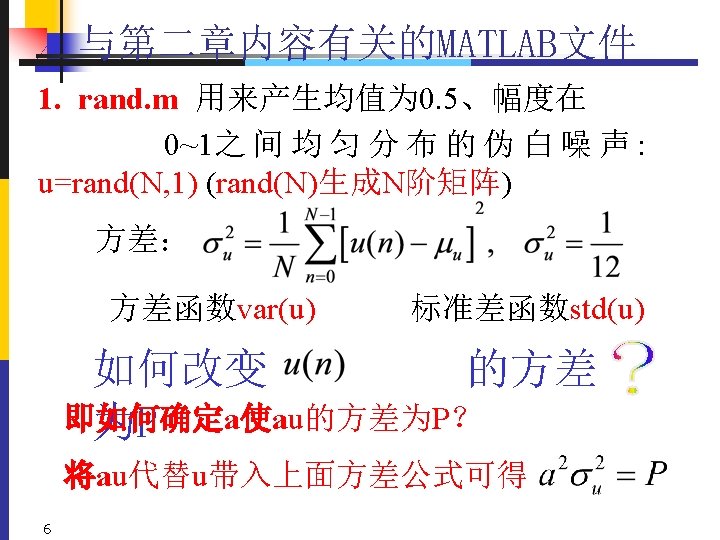
与信号处理间接有关的 具箱: Control System Communication (控制系统) (通信) System Identification (系统辨识) Statistics Neural Network 4 (统计) (神经网络)
;")
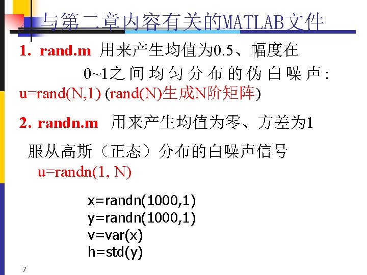
例: 5 z=peaks; surf(z);


 求“时域”函数ft的Fourier变换 uft=ifourier(Fw, w, t) 求“频域”函数Fw的Fourier 反变换 Laplace变换及其反变换 u.")
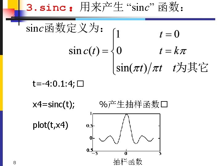
符号变换 Fourier变换及其反变换 u. Fw=fourier(ft, t, w) 求“时域”函数ft的Fourier变换 uft=ifourier(Fw, w, t) 求“频域”函数Fw的Fourier 反变换 Laplace变换及其反变换 u. Fs=laplace(ft, t, s) 求“时域”函数ft的Laplace变换 uft=ilaplace(Fs, s, t) 求“频域”函数Fs的Laplace 反变换 14
求Fourier变换 syms t w ut=heaviside(t); UT=fourier(ut) UT = pi*dirac(w)-i/w (2)求Fourier反变换 Ut=ifourier(UT,")
【例 】求 的Fourier变换。 (1)求Fourier变换 syms t w ut=heaviside(t); UT=fourier(ut) UT = pi*dirac(w)-i/w (2)求Fourier反变换 Ut=ifourier(UT, w, t) Ut =heaviside(t) 15
; Ut=heaviside(t-b);")
【例2. 5 -4】求 的Laplace变换。 syms t s; syms a b positive; %不限定则无结果 Dt=dirac(t-a); Ut=heaviside(t-b); Mt=[Dt, Ut; exp(-a*t)*sin(b*t), t^2*exp(-t)]; MS=laplace(Mt, t, s) MS = [ exp(-s*a), exp(-s*b)/s] [ 1/b/((s+a)^2/b^2+1), 16 2/(s+1)^3]
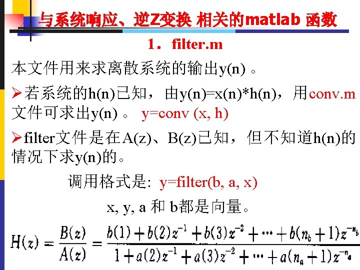
![7.deconv. m :实现系统的反卷积,其调用格式: [q, r]=deconv(y, x); 也用来实现多项式除法。 clear all; k=0: 1: 7; x=k+1; h=ones(1,](http://slidetodoc.com/presentation_image_h2/8eb4057e309df07461df5fac58392a9e/image-25.jpg "7.deconv. m :实现系统的反卷积,其调用格式: [q, r]=deconv(y, x); 也用来实现多项式除法。 clear all; k=0: 1: 7; x=k+1; h=ones(1,")
7.deconv. m :实现系统的反卷积,其调用格式: [q, r]=deconv(y, x); 也用来实现多项式除法。 clear all; k=0: 1: 7; x=k+1; h=ones(1, 4); y=conv(h, x); % y = x * h; [q, r]=deconv(y, x); % 由 y, x 作反卷积,求出 h; [q 1, r 1]=deconv(y, h); % 由 y, h 作反卷积,求出 x; subplot(321); stem(h, '. b'); ylabel(' h(n)'); subplot(322); stem(x, '. b'); ylabel(' x(n)'); subplot(323); stem(y, '. b'); ylabel(' y(n)'); subplot(325); stem(q, '. r'); ylabel(' q(n)'); subplot(326); stem(q 1, '. r'); ylabel(' q 1(n)'); clear all; % 实现多项式除法q=(4*x^3+1)/(2*x+1) y=[4 0 0 1]; x=[2 1]; [q, r]=deconv(y, x); → q=[2 -1 0. 5], r=[0 0 0 0. 5] 25
![例1: 系统 画出幅频响应及相频响应: 解: 转移函数: b=[1 -4 4]; a=[1]; [H, w]=freqz(b, a, 128, 'whole',](http://slidetodoc.com/presentation_image_h2/8eb4057e309df07461df5fac58392a9e/image-29.jpg "例1: 系统 画出幅频响应及相频响应: 解: 转移函数: b=[1 -4 4]; a=[1]; [H, w]=freqz(b, a, 128, 'whole',")
例1: 系统 画出幅频响应及相频响应: 解: 转移函数: b=[1 -4 4]; a=[1]; [H, w]=freqz(b, a, 128, 'whole', 1) Hr=abs(H); Hphase=angle(H); Hphaseu=unwrap(Hphase); subplot(311), plot(Hr) subplot(312), plot(Hphase) subplot(313), plot(Hphaseu) 29
![例2: b=[1]; a=[0, 1]; [H, w]=freqz(b, a, 256, 'whole', 1); Hr=abs(H); Hphase=angle(H); Hphase 1=unwrap(Hphase);](http://slidetodoc.com/presentation_image_h2/8eb4057e309df07461df5fac58392a9e/image-30.jpg "例2: b=[1]; a=[0, 1]; [H, w]=freqz(b, a, 256, 'whole', 1); Hr=abs(H); Hphase=angle(H); Hphase 1=unwrap(Hphase);")
例2: b=[1]; a=[0, 1]; [H, w]=freqz(b, a, 256, 'whole', 1); Hr=abs(H); Hphase=angle(H); Hphase 1=unwrap(Hphase); 解: 相位的卷绕 (wrapping) 解卷绕 30 画出幅频响应及相频响应:
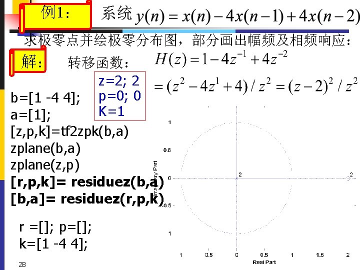
![例: 给定系统 求:极-零图 解:b=[. 1836. 7344 1. 1016. 7374. 1836]/100 a =[1 -3. 0544](http://slidetodoc.com/presentation_image_h2/8eb4057e309df07461df5fac58392a9e/image-31.jpg "例: 给定系统 求:极-零图 解:b=[. 1836. 7344 1. 1016. 7374. 1836]/100 a =[1 -3. 0544")
例: 给定系统 求:极-零图 解:b=[. 1836. 7344 1. 1016. 7374. 1836]/100 a =[1 -3. 0544 3. 8291 -2. 2925. 55075] 单位抽样响应 zplane(b, a); 频率响应 部分分式展开 [h, t]=impz(b, a, 40); stem(t, h, '. '); grid on; [H, w]=freqz(b, a, 256, 'whole', 1); Hr=abs(H); [r, p, k]= residuez(b, a) Hphase=angle(H); [b, a]= residuez(r, p, k) Hphase=unwrap(Hphase); 31
; 极-零图")
32 zplane(b, a); 极-零图
![[h, t]=impz(b, a, 40); stem(t, h, '. '); grid on; 单位抽样响应 33](http://slidetodoc.com/presentation_image_h2/8eb4057e309df07461df5fac58392a9e/image-33.jpg "[h, t]=impz(b, a, 40); stem(t, h, '. '); grid on; 单位抽样响应 33")
[h, t]=impz(b, a, 40); stem(t, h, '. '); grid on; 单位抽样响应 33
![[H, w]=freqz(b, a, 256, 'whole', 1); Hr=abs(H); subplot(311), plot(Hr) subplot(312), plot(Hphase) subplot(313), plot(Hphaseu) Hphase=angle(H);](http://slidetodoc.com/presentation_image_h2/8eb4057e309df07461df5fac58392a9e/image-34.jpg "[H, w]=freqz(b, a, 256, 'whole', 1); Hr=abs(H); subplot(311), plot(Hr) subplot(312), plot(Hphase) subplot(313), plot(Hphaseu) Hphase=angle(H);")
[H, w]=freqz(b, a, 256, 'whole', 1); Hr=abs(H); subplot(311), plot(Hr) subplot(312), plot(Hphase) subplot(313), plot(Hphaseu) Hphase=angle(H); Hphaseu=unwrap(Hphase); 34 频率响应
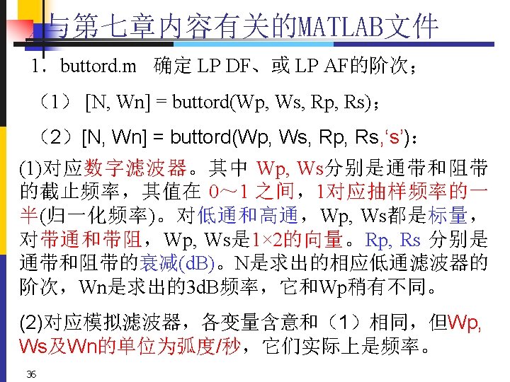
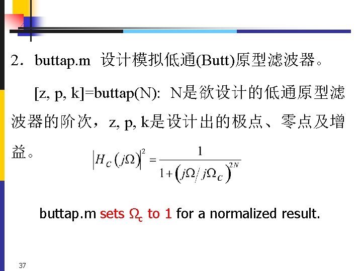

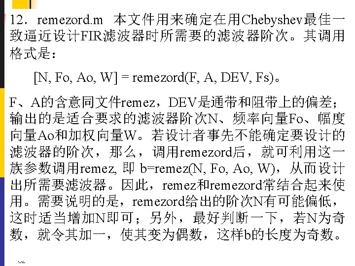
9.cheb 2 ord. m; 10. cheb 2 ap. m; 11. cheby 2. m; 12. ellipord. m; 对应 Cheby-II、 椭圆 IIR 滤波器 13. ellipap. m; 14. ellip. m; 15.impinvar. m 用冲激响应不变法实现频率转换; 42

例7. 1 设计 IIR LP DF, u clear all; fp=100; fs=300; Fs=1000; rp=3; rs=20; u wp=2*pi*fp/Fs; ws=2*pi*fs/Fs; u Fs=Fs/Fs; % let Fs=1 u % frequency prewarping ; u wap=2*Fs*tan(wp/2); was=2*Fs*tan(ws/2); % u [n, wn]=buttord(wap, was, rp, rs, 's') % Note: 's'! u [z, p, k]=buttap(n); % u [bp, ap]=zp 2 tf(z, p, k) % u [bs, as]=lp 2 lp(bp, ap, wn) % u [bz, az]=bilinear(bs, as, Fs) %% s=(2/Ts)(z-1)/(z+1); u [h, w]=freqz(bz, az, 256, Fs*1000); u plot(w, 20*log 10(abs(h))); grid on; 46

例7. 1 设计 IIR LP DF, uclear all; wp=. 2*pi; ws=. 6*pi; Fs=1000; rp=3; rs=20; u% frequency prewarping; uwap=2*Fs*tan(wp/2); was=2*Fs*tan(ws/2); u[n, wn]=buttord(wap, was, rp, rs, 's'); % Note: 's'! u[z, p, k]=buttap(n); u[bp, ap]=zp 2 tf(z, p, k); 模拟滤波器和数字滤 u[bs, as]=lp 2 lp(bp, ap, wap) 波器幅频特性比较 uw 1=[0: 499]*2*pi; uh 1=freqs(bs, as, w 1); u[bz, az]=bilinear(bs, as, Fs) % z=(2/ts)(z-1)/(z+1); u[h 2, w 2]=freqz(bz, az, 500, Fs); uplot(w 1/2/pi, abs(h 1), w 2, abs(h 2), 'k'); grid on; 47

例7. 1 设计 IIR LP DF, uclear all; uwp=. 2*pi; ws=. 6*pi; Fs=1000; urp=3; rs=20; u[n, wn]=buttord(wp/pi, ws/pi, rp, rs); u[bz, az]=butter(n, wp/pi) 保证通带上限指标满足 u[bz 1, az 1]=butter(n, wn) 保证阻带下限指标满足 u[h, w]=freqz(bz, az, 128, Fs); u[h 1, w 1]=freqz(bz 1, az 1, 128, Fs); uplot(w, 20*log 10(abs(h) ), w 1, 20*log 10(abs(h 1) ), 'g. '); ugrid on; 48

例7. 2 用matlab设计一FIR滤波器,要求频率指标如下: Solution: clc; clear all; close all wp=0. 15*pi; ws=0. 25*pi; Hanning窗 wdelta=ws-wp; N=ceil(8*pi/wdelta); Wn=(0. 15+0. 25)*pi/2; b=fir 1(N, Wn/pi, hanning(N+1)); figure % freqz(b, 1, 512) [H, w]=freqz(b, 1, 512) ; plot(w, abs(H)) set(gca, 'XTick', 0: 0. 2*pi: pi) set(gca, 'XTick. Label', {'0', '0. 2π', '0. 4π', '0. 6π', '0. 8π', 'π'}) axis([0, pi, 0. 97, 1. 03]); 52
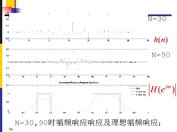
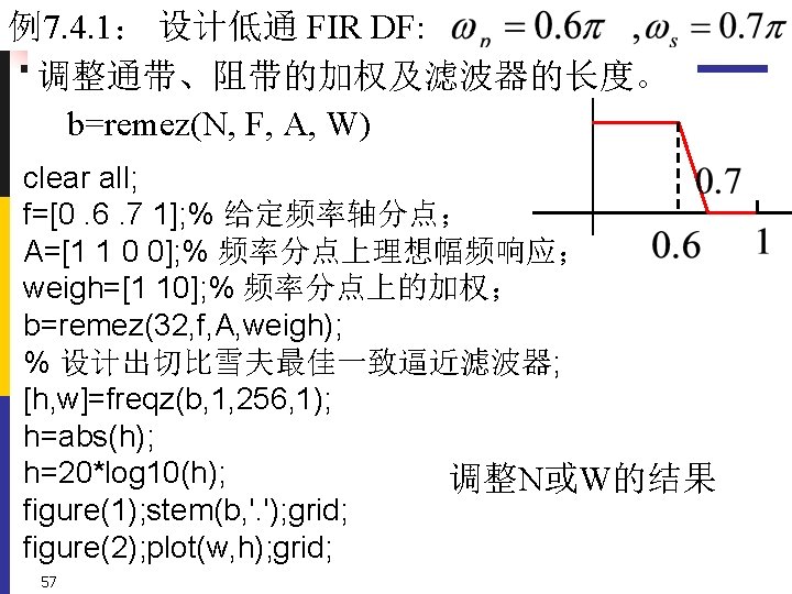
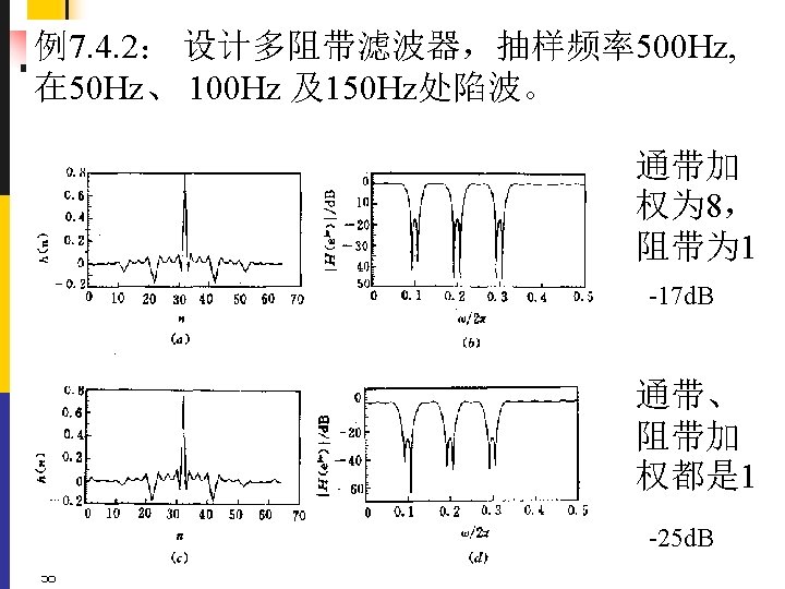

例7. 4. 2: 设计多阻带滤波器,抽样频率500 Hz, 在 50 Hz、 100 Hz 及150 Hz处陷波。 250 Hz clear all; f=[0. 14. 18. 22. 26. 34. 38. 42. 46. 54. 58. 62. 66 1]; A=[1 1 0 0 1 1]; weigh 1=[8 1 8 1 8]; b 1=remez(64, f, A, weigh 1); [h 1, w 1]=freqz(b 1, 1, 256, 1); h 1=abs(h 1); h 1=20*log 10(h 1); subplot(211); plot(w 1, h 1); grid; axis([0 0. 5 -60 10]) title('N=32, weight=[8 1 8 1 8]', 'Font. Size', 14, 'Color', 'r') 59

例7. 1. 1. 设计低通 DF FIR, 令截止频率 = 0. 25π, 取 M= 10, 20,40,观察其幅频响应的特点. clear all; N=10; b 1=fir 1(N, 0. 25, boxcar(N+1)); b 3=fir 1(2*N, 0. 25, boxcar(2*N+1)); b 4=fir 1(4*N, 0. 25, boxcar(4*N+1)); M=128; h 1=freqz(b 1, 1, M); h 3=freqz(b 3, 1, M); h 4=freqz(b 4, 1, M); f=0: 0. 5/M: 0. 5 -0. 5/M; plot(f, abs(h 1), f, abs(h 3), f, abs(h 4)); grid; axis([0 0. 5 0 1. 2]) 60

clear all; N=40; n=0: N; 例7. 1. 2: 理想差 b 1=fir 1(N, 0. 25, boxcar(N+1)); 分器及其设计 b 2=fir 1(N, 0. 25, hamming(N+1)); win=hamming(N+1); for n=1: N+1 if (n-1 -N/2)==0; b 1(n)=0; else M=128; b 1(n)=(-1)^(n-1 -N/2)/(n-1 -N/2); h 1=freqz(b 1, 1, M); end h 2=freqz(b 2, 1, M); end % h=freqz(b, 1, M); for n=1: N+1 f=0: 0. 5/M: 0. 5 -0. 5/M; if (n-1 -N/2)==0; hd=2*pi*f; b 2(n)=0; plot(f, abs(h 1), f, abs(h 2), f, hd, 'k-') else b 2(n)=win(n)*(-1)^(n-1 -N/2)/(n-1 -N/2); end 61
 fftshift(X) 64")
信号x X=fft(x) fftshift(X) 64
是两个正弦信号及白噪声的叠加,进行频 谱分析。 clear all; % 产生两个正弦加白噪声; N=256; f 1=. 1; f")
• 例1. 设x(n)是两个正弦信号及白噪声的叠加,进行频 谱分析。 clear all; % 产生两个正弦加白噪声; N=256; f 1=. 1; f 2=. 2; fs=1; a 1=5; a 2=3; w=2*pi/fs; x=a 1*sin(w*f 1*(0: N-1))+a 2*sin(w*f 2*(0: N-1))+randn(1, N); % 应用FFT 求频谱; subplot(4, 1, 1); plot(x(1: N/4)); axis tight f 1=0: 2*pi/N: 2*pi-pi/N; f=-pi: 2*pi/N: pi-pi/N; X=fft(x); y=ifft(X); subplot(4, 1, 2); plot(f 1, abs(X)); axis tight subplot(4, 1, 3); plot(f, fftshift(abs(X))); axis tight subplot(4, 1, 4); plot(real(y(1: N/4))); axis tight 66
 fftshift(X) x’=ifft(X) 67")
信号x X=fft(x) fftshift(X) x’=ifft(X) 67
为一正弦加白噪声信号,长度为 500,h(n)是 用fir 1. m文件设计的一个低通FIR滤波器,长度为 11. 试 用fftfilt实现长序列的卷积 clear; % 用叠接相加法,计算滤波器系数h和输入信号x的卷积 % 其中h为")
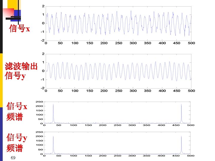
例2 令x(n)为一正弦加白噪声信号,长度为 500,h(n)是 用fir 1. m文件设计的一个低通FIR滤波器,长度为 11. 试 用fftfilt实现长序列的卷积 clear; % 用叠接相加法,计算滤波器系数h和输入信号x的卷积 % 其中h为 10阶hanning窗,x是带有高斯白噪的正弦信号 h=fir 1(10, 0. 3, hanning(11)); % h: is the impulse response of a N=500; p=0. 05; f=1/16; % low-pass filter. u=randn(1, N)*sqrt(p); % u: white noise s=sin(2*pi*f*[0: N-1]); % s: sine signal x=u(1: N)+s; % x: a long sequence; y=fftfilt(h, x); % Overlap-add method of FIR filtering using FFT % y=filter(h, 1, x); % y=x*h subplot(211); plot(x); subplot(212); plot(y); figure; subplot(211); plot(abs(fft(x))); 68 subplot(212); plot(abs(fft(y)));
); N=500; p=0. 05; f=1/16;")
clear; % 按照overlap-add算法编程实现长信号滤波输出 % 生成滤波器系数h和混有高斯白噪的正弦信号x h=fir 1(10, 0. 3, hanning(11)); N=500; p=0. 05; f=1/16; u=randn(1, N)*sqrt(p); % s=sin(2*pi*f*[0: N-1]); x=u(1: N)+s; % 将x分为长度为L的小段 L=20; M=length(h); y=zeros(1, N+M-1); tempy=zeros(1, M+L-1); temp. X=zeros(1, L); for k=0: N/L-1 tempx(1: L)=x(k*L+1: (k+1)*L); tempy=conv(tempx, h); y=y+[zeros(1, k*L), tempy, zeros(1, N-(k+1)*L)]; end subplot(211); plot(x) subplot(212); plot(y(1: N)) 70

71
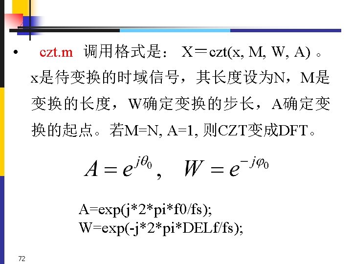
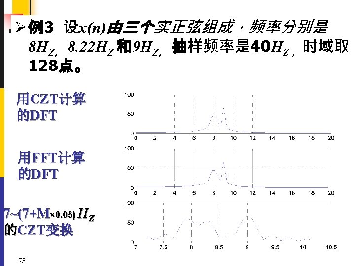

• 程序 clear all; % 构造三个不同频率的正弦信号的叠加作为试验信号 N=128; f 1=8; f 2=8. 22; f 3=9; fs=40; stepf=fs/N; n=0: N-1; t=2*pi*n/fs; n 1=0: stepf: fs/2 -stepf; x=sin(f 1*t)+sin(f 2*t)+sin(f 3*t); M=N; W=exp(-j*2*pi/M); % A=1时的czt变换 A=1; Y 1=czt(x, M, W, A); subplot(311) plot(n 1, abs(Y 1(1: N/2))); grid on; 74
); subplot(312) plot(n 1, abs(Y 2(1: N/2))); grid on; % 详细构造A后的czt")
% DFT Y 2=abs(fft(x)); subplot(312) plot(n 1, abs(Y 2(1: N/2))); grid on; % 详细构造A后的czt M=60; f 0=7. 2; DELf=0. 05; A=exp(j*2*pi*f 0/fs); W=exp(-j*2*pi*DELf/fs); Y 3=czt(x, M, W, A); n 2=f 0: DELf: f 0+(M-1)*DELf; subplot(313); plot(n 2, abs(Y 3)); grid on; 75
- Slides: 76