Biomedical Signal processing Chapter 2 DiscreteTime Signals and

Biomedical Signal processing Chapter 2 Discrete-Time Signals and Systems Zhongguo Liu Biomedical Engineering School of Control Science and Engineering, Shandong University 山东省精品课程《生物医学信号处理(双语)》 http: //course. sdu. edu. cn/bdsp. html 2021/12/18 1 1 Zhongguo Liu_Biomedical Engineering_Shandong Univ.

Chapter 2 Discrete-Time Signals and Systems u 2. 0 Introduction u 2. 1 Discrete-Time Signals: Sequences u 2. 2 Discrete-Time Systems u 2. 3 Linear Time-Invariant (LTI) Systems u 2. 4 Properties of LTI Systems u 2. 5 Linear Constant-Coefficient Difference Equations 2 12/18/2021 Zhongguo Liu_Biomedical Engineering_Shandong Univ.

Chapter 2 Discrete-Time Signals and Systems u 2. 6 Frequency-Domain Representation of Discrete-Time Signals and systems u 2. 7 Representation of Sequences by Fourier Transforms u 2. 8 Symmetry Properties of the Fourier Transform u 2. 9 Fourier Transform Theorems u 2. 10 Discrete-Time Random Signals u 2. 11 Summary 3 12/18/2021 Zhongguo Liu_Biomedical Engineering_Shandong Univ.

2. 0 Introduction u. Signal: something conveys information, represented mathematically as functions of one or more independent variables. Classified as: u. Continuous-time (analog) signals, discrete-time signals, digital signals u. Signal-processing systems are classified along the same lines as signals: Continuous-time (analog) systems, discrete-time systems, digital systems 4 12/18/2021 Zhongguo Liu_Biomedical Engineering_Shandong Univ.

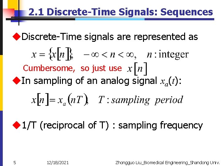
2. 1 Discrete-Time Signals: Sequences u. Discrete-Time signals are represented as Cumbersome, so just use u. In sampling of an analog signal xa(t): u 1/T (reciprocal of T) : sampling frequency 5 12/18/2021 Zhongguo Liu_Biomedical Engineering_Shandong Univ.

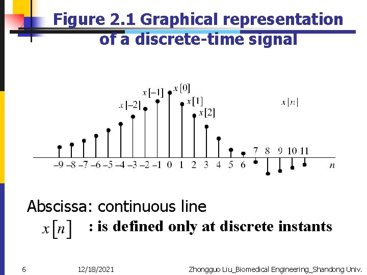
Figure 2. 1 Graphical representation of a discrete-time signal Abscissa: continuous line : is defined only at discrete instants 6 12/18/2021 Zhongguo Liu_Biomedical Engineering_Shandong Univ.

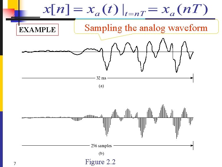
EXAMPLE 7 Sampling the analog waveform Figure 2. 2

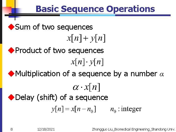
Basic Sequence Operations u. Sum of two sequences u. Product of two sequences u. Multiplication of a sequence by a number α u. Delay (shift) of a sequence 8 12/18/2021 Zhongguo Liu_Biomedical Engineering_Shandong Univ.

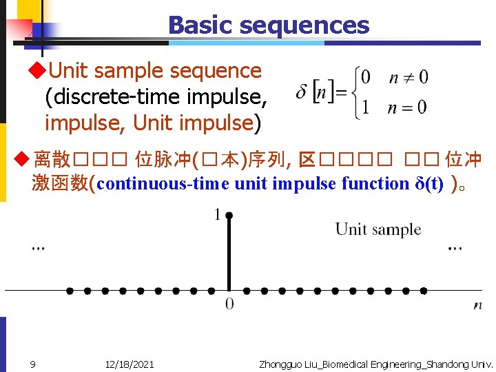
Basic sequences u. Unit sample sequence (discrete-time impulse, Unit impulse) u离散��� 位脉冲(� 本)序列, 区���� �� 位冲 激函数(continuous-time unit impulse function δ(t) )。 9 12/18/2021 Zhongguo Liu_Biomedical Engineering_Shandong Univ.

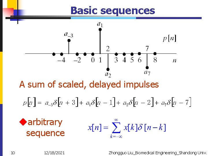
Basic sequences A sum of scaled, delayed impulses uarbitrary sequence 10 12/18/2021 Zhongguo Liu_Biomedical Engineering_Shandong Univ.

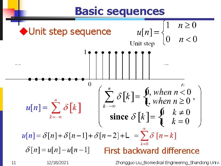
Basic sequences u. Unit step sequence First backward difference 11 12/18/2021 Zhongguo Liu_Biomedical Engineering_Shandong Univ.

Basic Sequences u. Exponential sequences u. A and α are real: x[n] is real u. A is positive and 0<α<1, x[n] is positive and decrease with increasing n u-1<α<0, x[n] alternate in sign, but decrease in magnitude with increasing n u : x[n] grows in magnitude as n increases 12 12/18/2021 Zhongguo Liu_Biomedical Engineering_Shandong Univ.

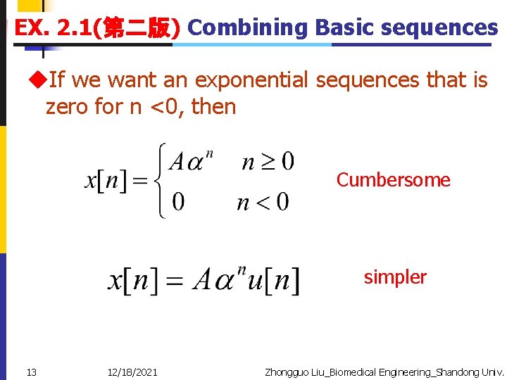
EX. 2. 1(第二版) Combining Basic sequences u. If we want an exponential sequences that is zero for n <0, then Cumbersome simpler 13 12/18/2021 Zhongguo Liu_Biomedical Engineering_Shandong Univ.

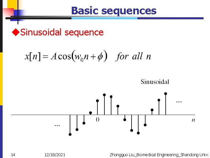
Basic sequences u. Sinusoidal sequence 14 12/18/2021 Zhongguo Liu_Biomedical Engineering_Shandong Univ.

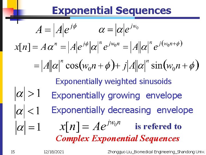
Exponential Sequences Exponentially weighted sinusoids Exponentially growing envelope Exponentially decreasing envelope is refered to Complex Exponential Sequences 15 12/18/2021 Zhongguo Liu_Biomedical Engineering_Shandong Univ.

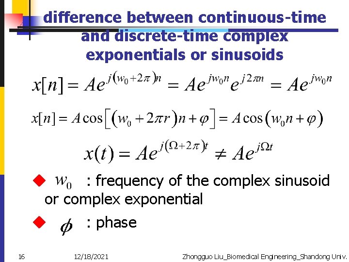
difference between continuous-time and discrete-time complex exponentials or sinusoids u : frequency of the complex sinusoid or complex exponential u : phase 16 12/18/2021 Zhongguo Liu_Biomedical Engineering_Shandong Univ.

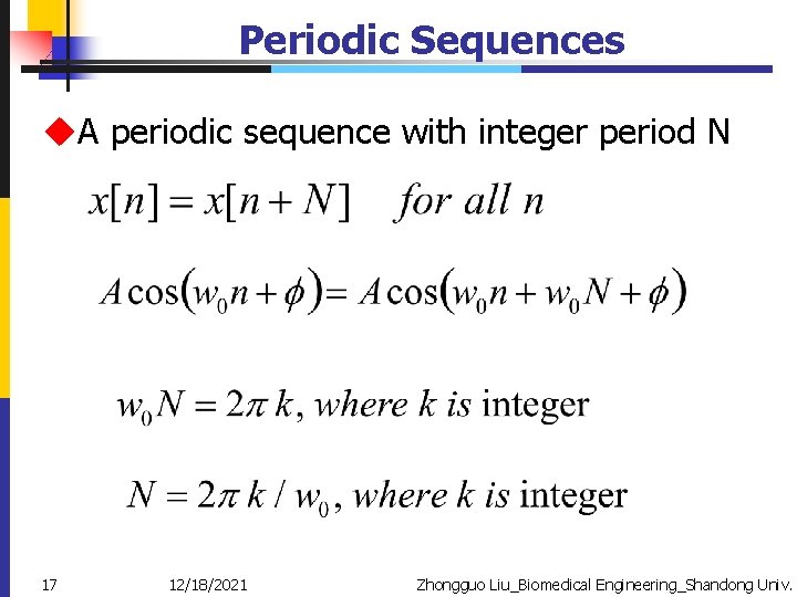
Periodic Sequences u. A periodic sequence with integer period N 17 12/18/2021 Zhongguo Liu_Biomedical Engineering_Shandong Univ.

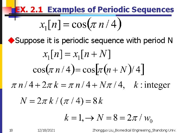
EX. 2. 1 Examples of Periodic Sequences u. Suppose it is periodic sequence with period N 18 12/18/2021 Zhongguo Liu_Biomedical Engineering_Shandong Univ.

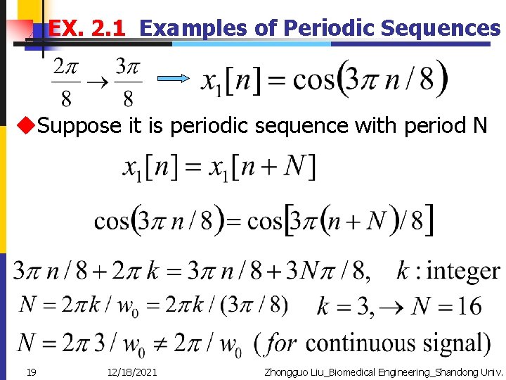
EX. 2. 1 Examples of Periodic Sequences u. Suppose it is periodic sequence with period N 19 12/18/2021 Zhongguo Liu_Biomedical Engineering_Shandong Univ.

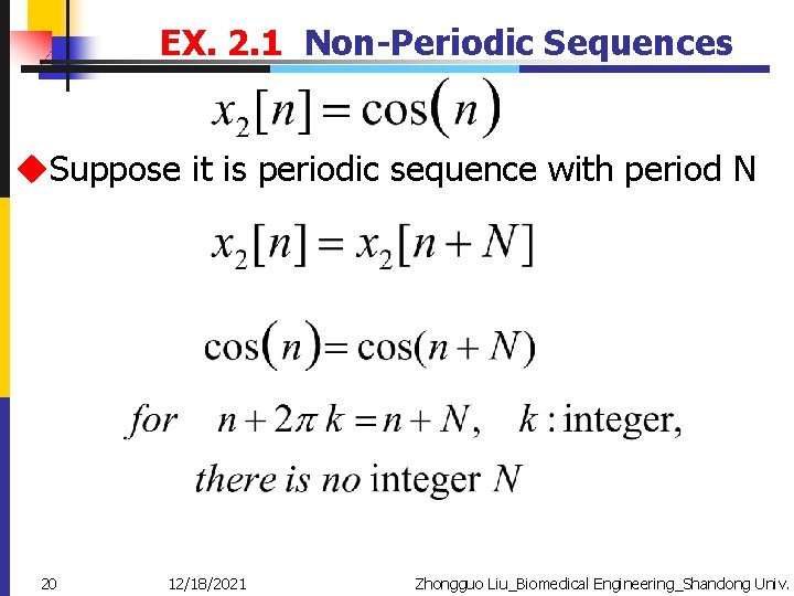
EX. 2. 1 Non-Periodic Sequences u. Suppose it is periodic sequence with period N 20 12/18/2021 Zhongguo Liu_Biomedical Engineering_Shandong Univ.

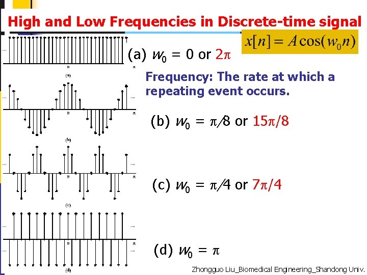
High and Low Frequencies in Discrete-time signal (a) w 0 = 0 or 2 Frequency: The rate at which a repeating event occurs. (b) w 0 = /8 or 15 /8 (c) w 0 = /4 or 7 /4 (d) w 0 = 21 12/18/2021 Zhongguo Liu_Biomedical Engineering_Shandong Univ.

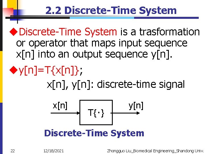
2. 2 Discrete-Time System u. Discrete-Time System is a trasformation or operator that maps input sequence x[n] into an output sequence y[n]. uy[n]=T{x[n]}; x[n], y[n]: discrete-time signal x[n] T{‧} y[n] Discrete-Time System 22 12/18/2021 Zhongguo Liu_Biomedical Engineering_Shandong Univ.

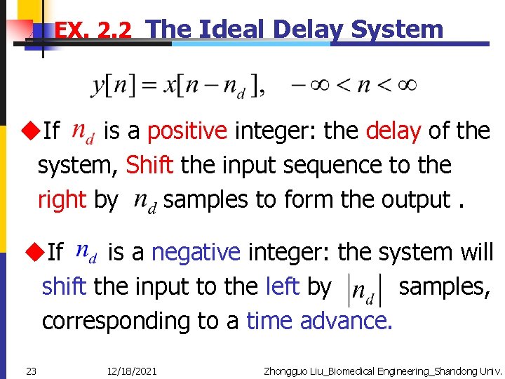
EX. 2. 2 The Ideal Delay System u. If is a positive integer: the delay of the system, Shift the input sequence to the right by samples to form the output. u. If is a negative integer: the system will shift the input to the left by samples, corresponding to a time advance. 23 12/18/2021 Zhongguo Liu_Biomedical Engineering_Shandong Univ.

EX. 2. 3 Moving Average for n=7, M 1=0, M 2=5 y[7] x[m] n-5 n 24 12/18/2021 m dummy index m Zhongguo Liu_Biomedical Engineering_Shandong Univ.

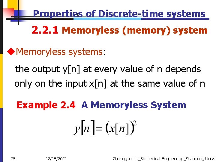
Properties of Discrete-time systems 2. 2. 1 Memoryless (memory) system u. Memoryless systems: the output y[n] at every value of n depends only on the input x[n] at the same value of n Example 2. 4 A Memoryless System 25 12/18/2021 Zhongguo Liu_Biomedical Engineering_Shandong Univ.

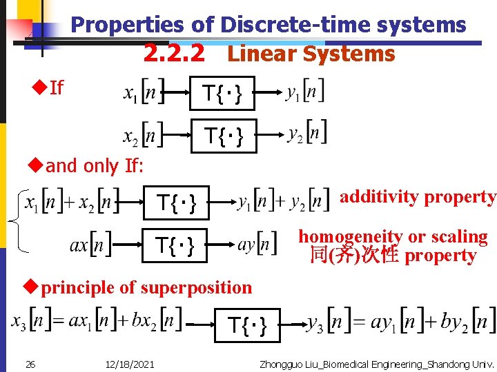
Properties of Discrete-time systems 2. 2. 2 Linear Systems u. If T{‧} uand only If: additivity property T{‧} homogeneity or scaling 同(齐)次性 property T{‧} uprinciple of superposition T{‧} 26 12/18/2021 Zhongguo Liu_Biomedical Engineering_Shandong Univ.

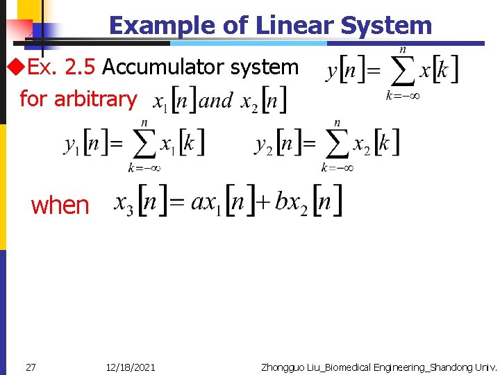
Example of Linear System u. Ex. 2. 5 Accumulator system for arbitrary when 27 12/18/2021 Zhongguo Liu_Biomedical Engineering_Shandong Univ.

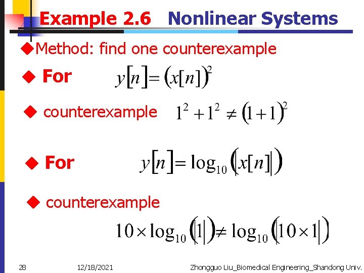
Example 2. 6 Nonlinear Systems u. Method: find one counterexample u For u counterexample 28 12/18/2021 Zhongguo Liu_Biomedical Engineering_Shandong Univ.

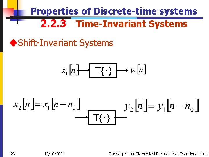
Properties of Discrete-time systems 2. 2. 3 Time-Invariant Systems u. Shift-Invariant Systems T{‧} 29 12/18/2021 Zhongguo Liu_Biomedical Engineering_Shandong Univ.

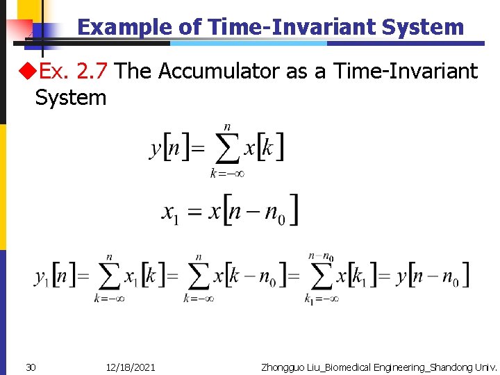
Example of Time-Invariant System u. Ex. 2. 7 The Accumulator as a Time-Invariant System 30 12/18/2021 Zhongguo Liu_Biomedical Engineering_Shandong Univ.

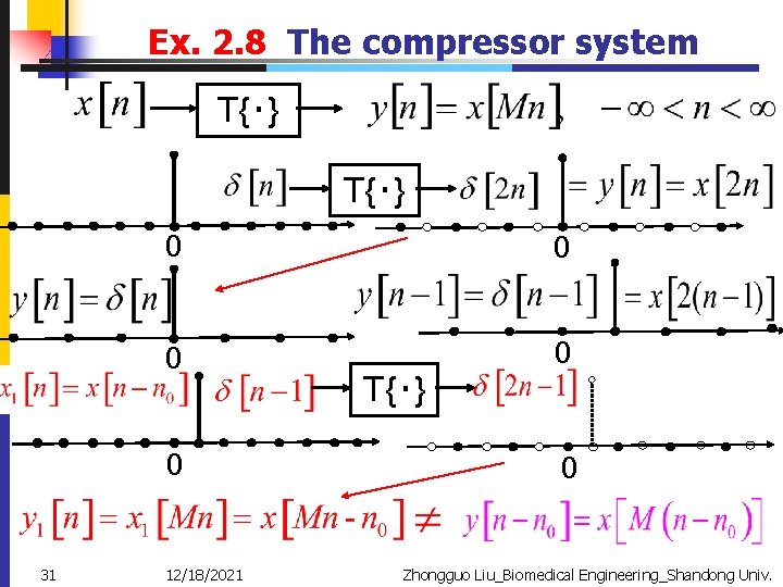
Ex. 2. 8 The compressor system T{‧} 0 0 0 31 12/18/2021 T{‧} 0 Zhongguo Liu_Biomedical Engineering_Shandong Univ.

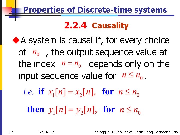
Properties of Discrete-time systems 2. 2. 4 Causality u. A system is causal if, for every choice of , the output sequence value at the index depends only on the input sequence value for. 32 12/18/2021 Zhongguo Liu_Biomedical Engineering_Shandong Univ.

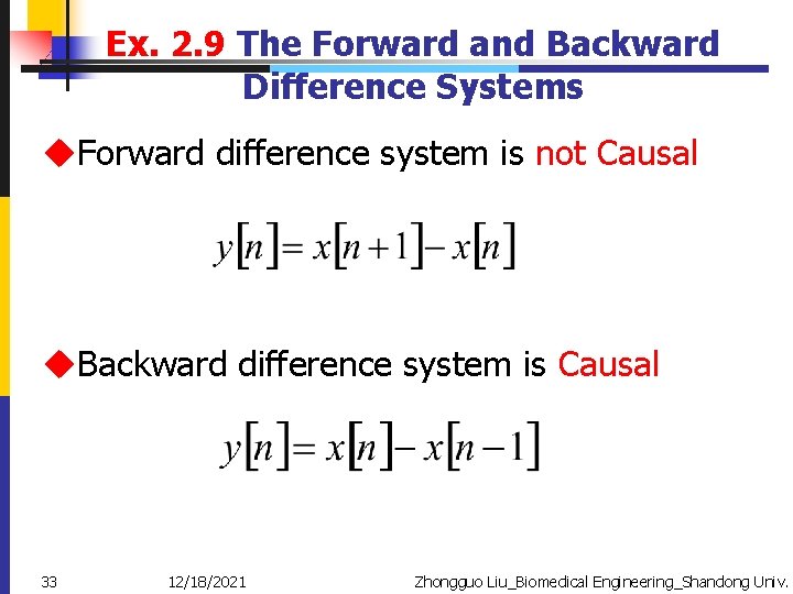
Ex. 2. 9 The Forward and Backward Difference Systems u. Forward difference system is not Causal u. Backward difference system is Causal 33 12/18/2021 Zhongguo Liu_Biomedical Engineering_Shandong Univ.

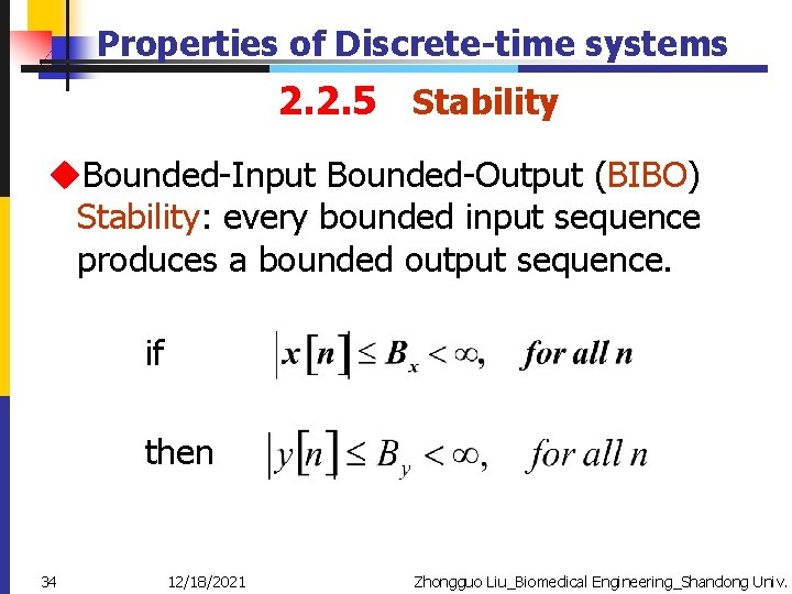
Properties of Discrete-time systems 2. 2. 5 Stability u. Bounded-Input Bounded-Output (BIBO) Stability: every bounded input sequence produces a bounded output sequence. if then 34 12/18/2021 Zhongguo Liu_Biomedical Engineering_Shandong Univ.

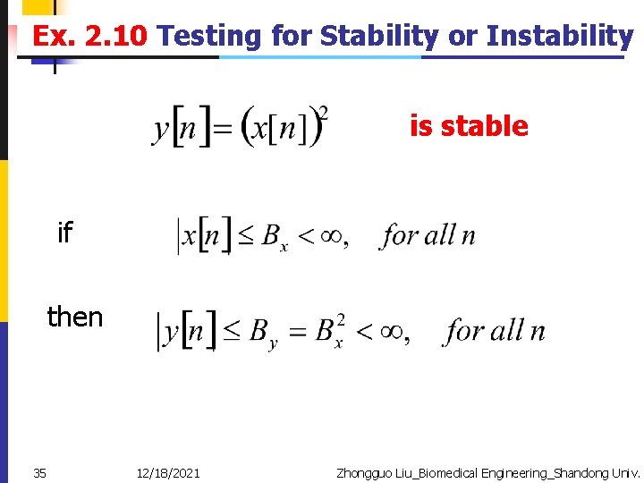
Ex. 2. 10 Testing for Stability or Instability is stable if then 35 12/18/2021 Zhongguo Liu_Biomedical Engineering_Shandong Univ.

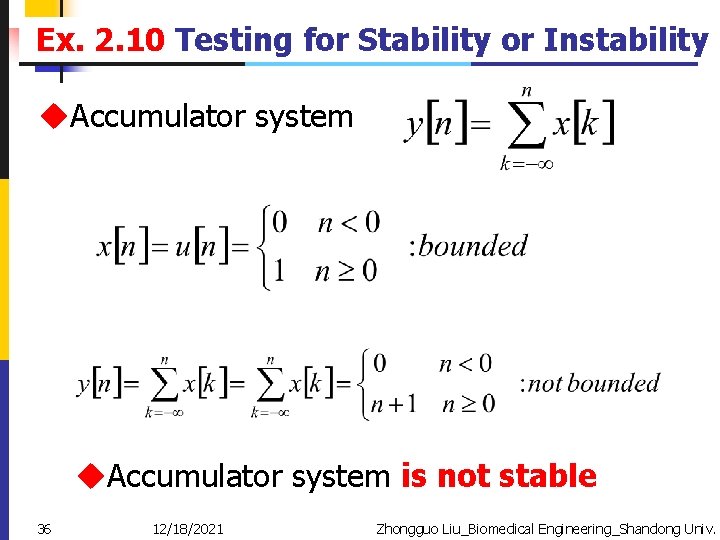
Ex. 2. 10 Testing for Stability or Instability u. Accumulator system is not stable 36 12/18/2021 Zhongguo Liu_Biomedical Engineering_Shandong Univ.

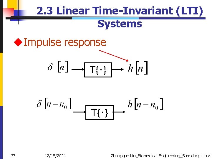
2. 3 Linear Time-Invariant (LTI) Systems u. Impulse response T{‧} 37 12/18/2021 Zhongguo Liu_Biomedical Engineering_Shandong Univ.

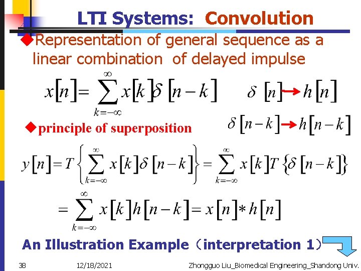
LTI Systems: Convolution u. Representation of general sequence as a linear combination of delayed impulse uprinciple of superposition An Illustration Example（interpretation 1） 38 12/18/2021 Zhongguo Liu_Biomedical Engineering_Shandong Univ.

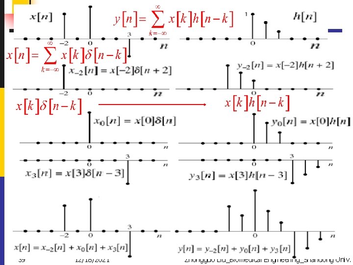
39 12/18/2021 Zhongguo Liu_Biomedical Engineering_Shandong Univ.

Computation of the Convolution （interpretation 2） ureflecting h[k] about the origion to obtain h[-k] u. Shifting the origin of the reflected sequence to k=n 40 12/18/2021 Zhongguo Liu_Biomedical Engineering_Shandong Univ.

Convolution can be realized by –Reflecting(reversing) h[k] about the origin to obtain h[-k]. –Shifting the origin of the reflected sequences to k=n. –Computing the weighted moving average of x[k] by using the weights given by h[n-k]. 41

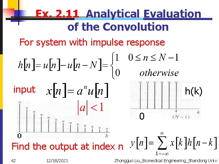
Ex. 2. 11 Analytical Evaluation of the Convolution For system with impulse response input h(k) 0 Find the output at index n 42 12/18/2021 Zhongguo Liu_Biomedical Engineering_Shandong Univ.

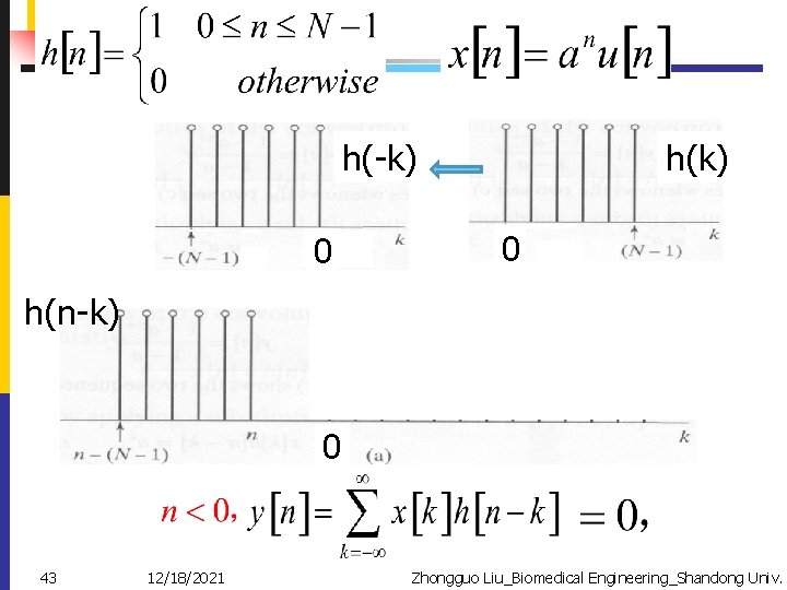
h(k) h(-k) 0 0 h(n-k) x(k) 0 43 12/18/2021 Zhongguo Liu_Biomedical Engineering_Shandong Univ.

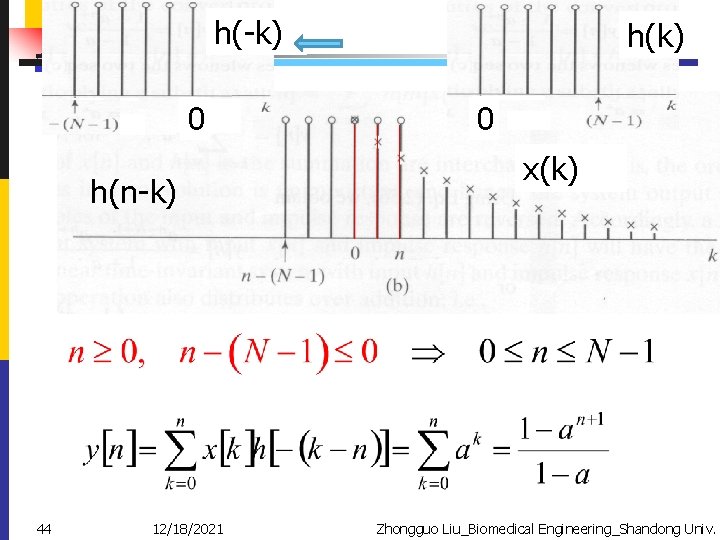
h(-k) 0 h(n-k) 44 12/18/2021 h(k) 0 x(k) Zhongguo Liu_Biomedical Engineering_Shandong Univ.

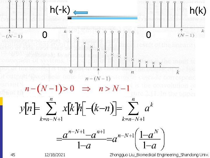
h(-k) 0 45 12/18/2021 h(k) 0 Zhongguo Liu_Biomedical Engineering_Shandong Univ.

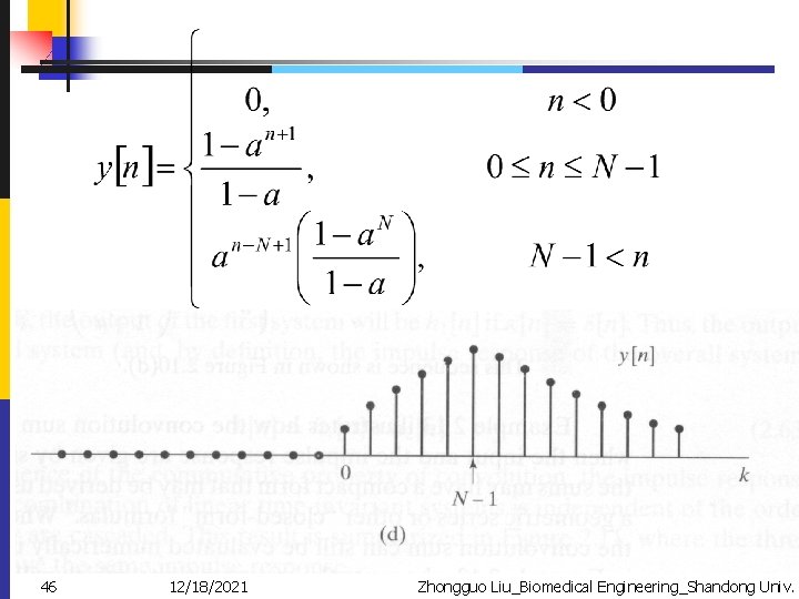
46 12/18/2021 Zhongguo Liu_Biomedical Engineering_Shandong Univ.

2. 4 Properties of LTI Systems u. Convolution is commutative(可交换的) x[n] h[n] y[n] h[n] x[n] y[n] u. Convolution is distributed over addition 47 12/18/2021 Zhongguo Liu_Biomedical Engineering_Shandong Univ.

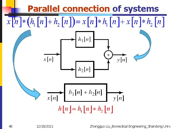
Parallel connection of systems 48 12/18/2021 Zhongguo Liu_Biomedical Engineering_Shandong Univ.

Cascade connection of systems associative property 结合性 commutative x [ n] h 1[ n] h 2[ n] y [ n] x [ n] h 2[ n] h 1[ n] y [ n] x [ n] 49 12/18/2021 h 1[n] ] h 2[n] y [ n] Zhongguo Liu_Biomedical Engineering_Shandong Univ.

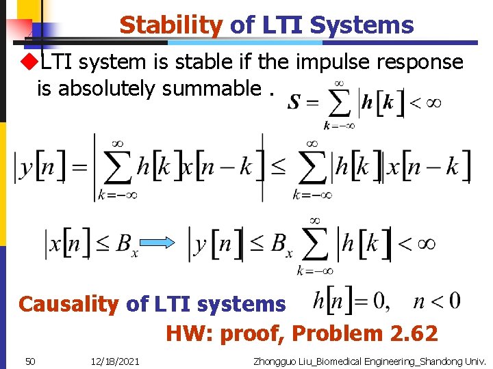
Stability of LTI Systems u. LTI system is stable if the impulse response is absolutely summable. Causality of LTI systems HW: proof, Problem 2. 62 50 12/18/2021 Zhongguo Liu_Biomedical Engineering_Shandong Univ.

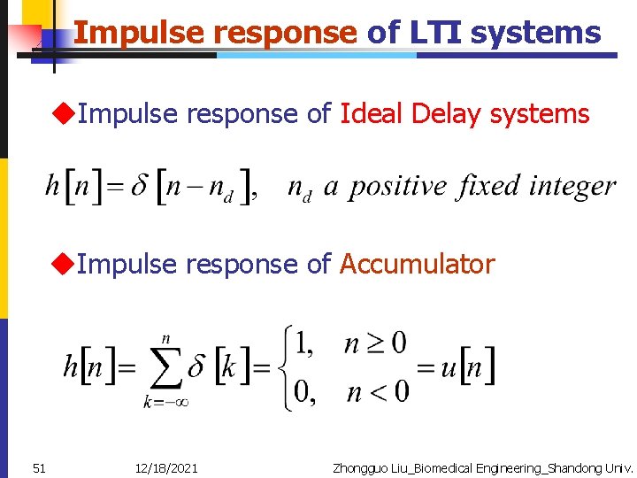
Impulse response of LTI systems u. Impulse response of Ideal Delay systems u. Impulse response of Accumulator 51 12/18/2021 Zhongguo Liu_Biomedical Engineering_Shandong Univ.

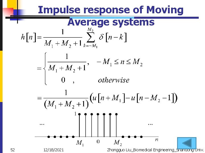
Impulse response of Moving Average systems 52 12/18/2021 Zhongguo Liu_Biomedical Engineering_Shandong Univ.

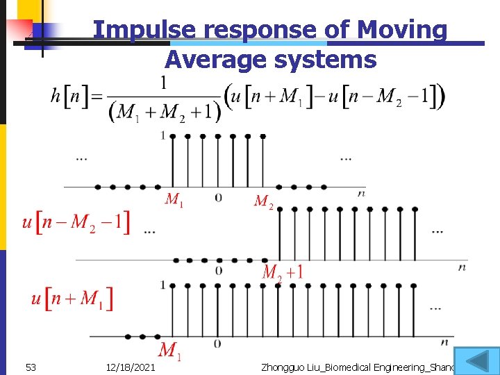
Impulse response of Moving Average systems 53 12/18/2021 Zhongguo Liu_Biomedical Engineering_Shandong Univ.

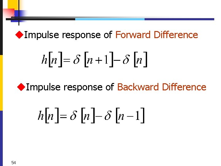
u. Impulse response of Forward Difference u. Impulse response of Backward Difference 54

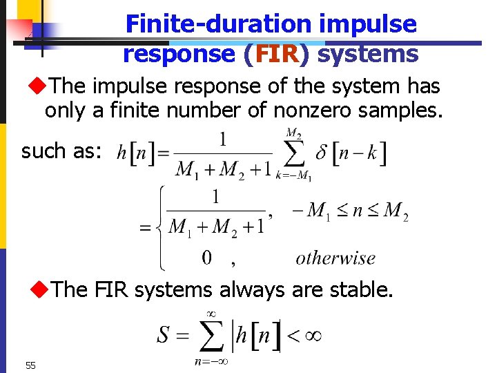
Finite-duration impulse response (FIR) systems u. The impulse response of the system has only a finite number of nonzero samples. such as: u. The FIR systems always are stable. 55

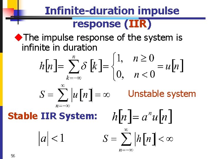
Infinite-duration impulse response (IIR) u. The impulse response of the system is infinite in duration Unstable system Stable IIR System: 56

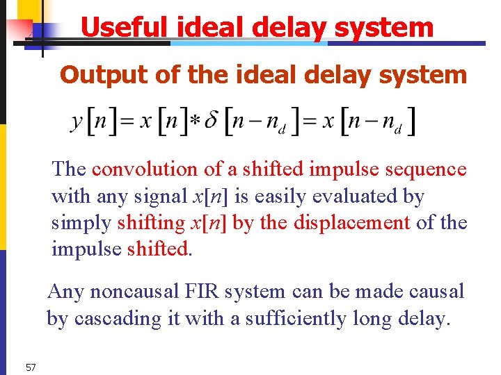
Useful ideal delay system Output of the ideal delay system The convolution of a shifted impulse sequence with any signal x[n] is easily evaluated by simply shifting x[n] by the displacement of the impulse shifted. Any noncausal FIR system can be made causal by cascading it with a sufficiently long delay. 57

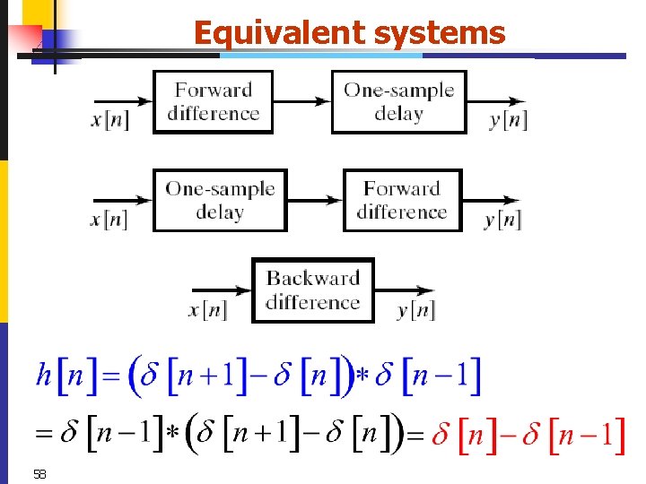
Equivalent systems 58

Inverse system x[n] hi[n] δ[n] 59 y[n]= x[n]*]= x[n]

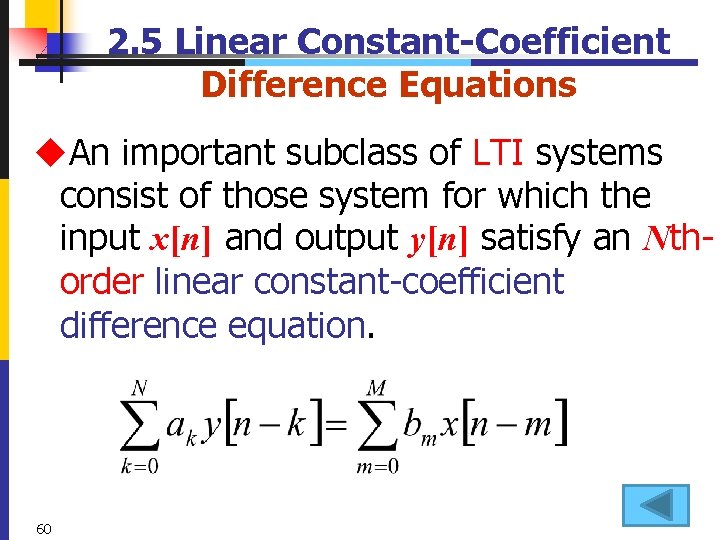
2. 5 Linear Constant-Coefficient Difference Equations u. An important subclass of LTI systems consist of those system for which the input x[n] and output y[n] satisfy an Nthorder linear constant-coefficient difference equation. 60

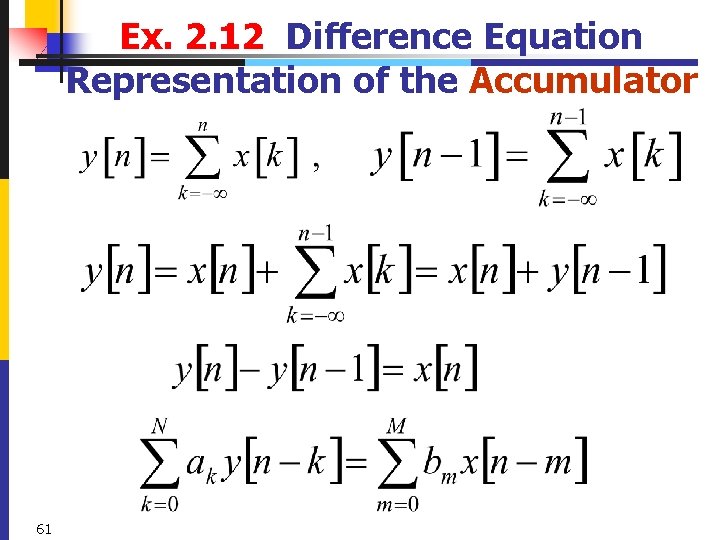
Ex. 2. 12 Difference Equation Representation of the Accumulator 61

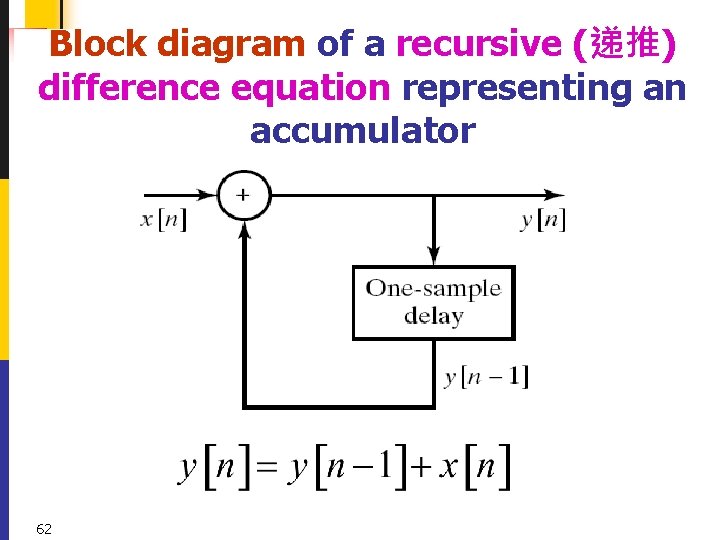
Block diagram of a recursive (递推) difference equation representing an accumulator 62

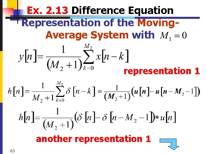
Ex. 2. 13 Difference Equation Representation of the Moving. Average System with representation 1 another representation 1 63

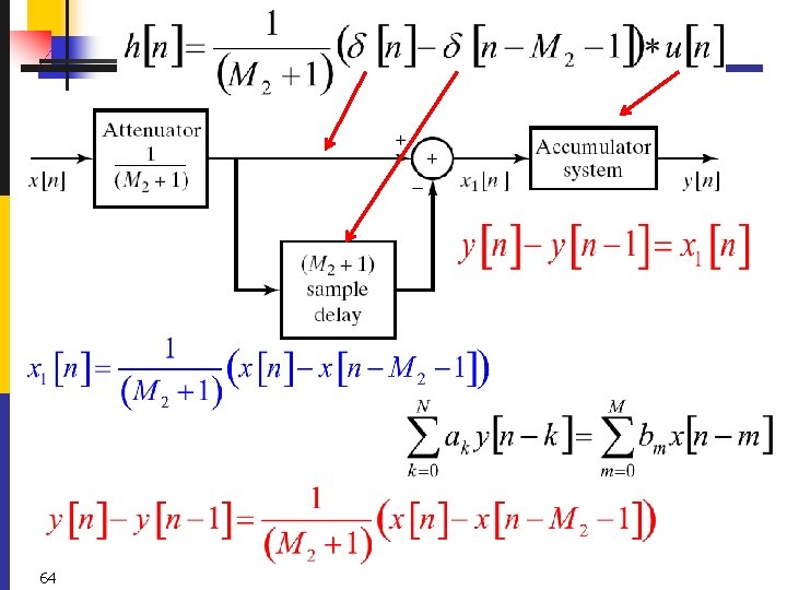
64

Difference Equation Representation of the System u. In Chapter 6, we will see that many (unlimited number of ) distinct difference equations can be used to represent a given linear time-invariant (LTI) input-output relation. 65

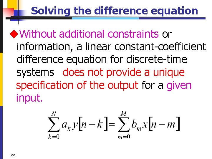
Solving the difference equation u. Without additional constraints or information, a linear constant-coefficient difference equation for discrete-time systems does not provide a unique specification of the output for a given input. 66

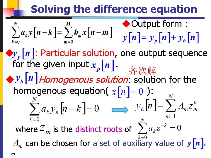
Solving the difference equation u. Output form : u : Particular solution, one output sequence for the given input. 齐次解 u Homogenous solution: solution for the homogenous equation( ): where is the distinct roots of can be chosen for a set of auxiliary value of 67

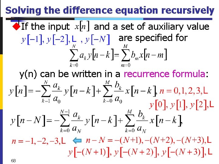
Solving the difference equation recursively u. If the input and a set of auxiliary value are specified for y(n) can be written in a recurrence formula: 68

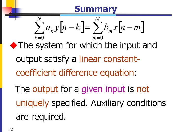
Summary u. The system for which the input and output satisfy a linear constantcoefficient difference equation: The output for a given input is not uniquely specified. Auxiliary conditions are required. 72

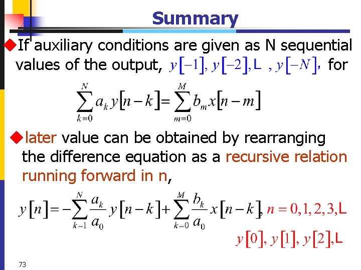
Summary u. If auxiliary conditions are given as N sequential values of the output, for ulater value can be obtained by rearranging the difference equation as a recursive relation running forward in n, 73

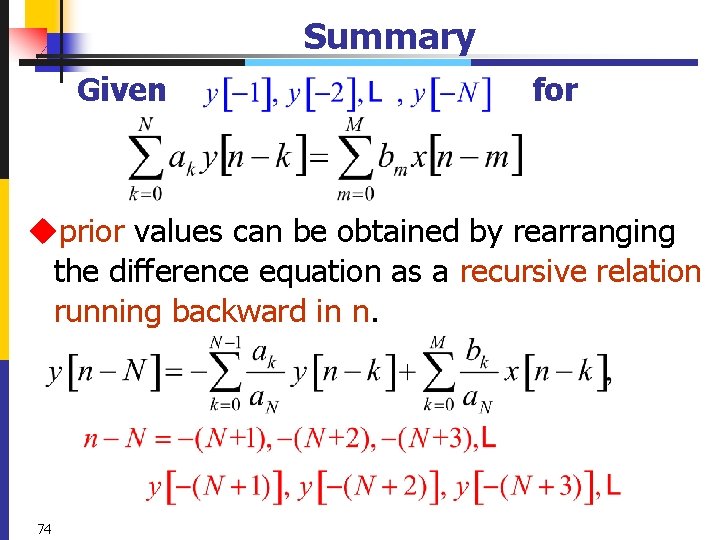
Summary Given for uprior values can be obtained by rearranging the difference equation as a recursive relation running backward in n. 74

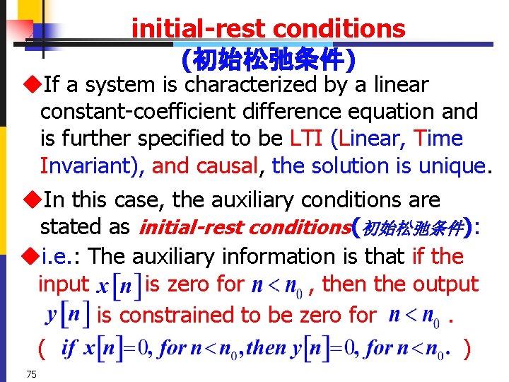
initial-rest conditions (初始松弛条件) u. If a system is characterized by a linear constant-coefficient difference equation and is further specified to be LTI (Linear, Time Invariant), and causal, the solution is unique. u. In this case, the auxiliary conditions are stated as initial-rest conditions(初始松弛条件): ui. e. : The auxiliary information is that if the input is zero for , then the output is constrained to be zero for. ( ) 75

Summary u. LTI (Linearity, Time Invariance), and causality of the system will depend on the auxiliary conditions. u. If an additional condition is that the system is initially at rest (初始松弛), then the system will be linear, time invariant, and causal. 76

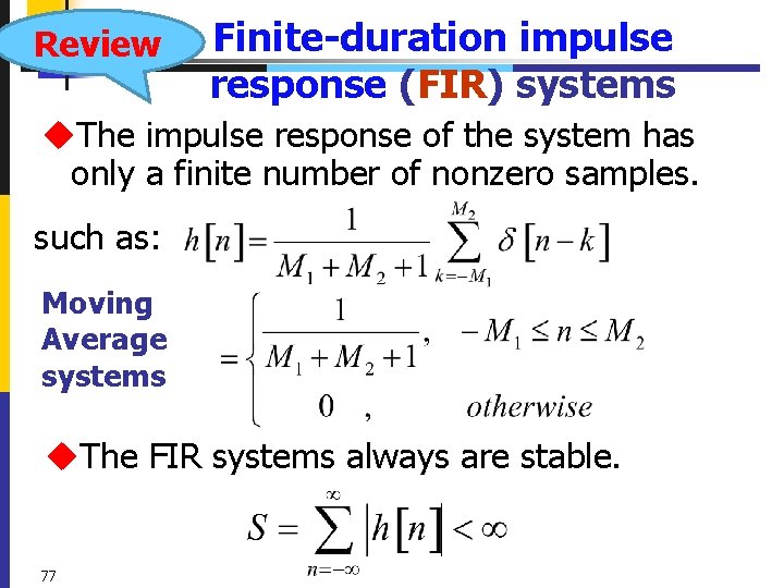
Review Finite-duration impulse response (FIR) systems u. The impulse response of the system has only a finite number of nonzero samples. such as: Moving Average systems u. The FIR systems always are stable. 77

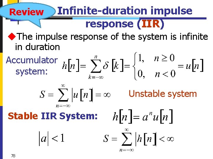
Review Infinite-duration impulse response (IIR) u. The impulse response of the system is infinite in duration Accumulator system: Unstable system Stable IIR System: 78

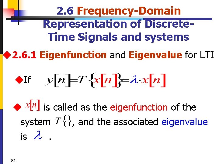
2. 6 Frequency-Domain Representation of Discrete. Time Signals and systems u 2. 6. 1 Eigenfunction and Eigenvalue for LTI u. If u is called as the eigenfunction of the system , and the associated eigenvalue is. 81

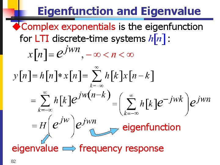
Eigenfunction and Eigenvalue u. Complex exponentials is the eigenfunction for LTI discrete-time systems : eigenfunction eigenvalue 82 frequency response

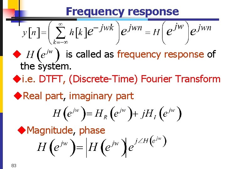
Frequency response u is called as frequency response of the system. ui. e. DTFT, (Discrete-Time) Fourier Transform u. Real part, imaginary part u. Magnitude, phase 83

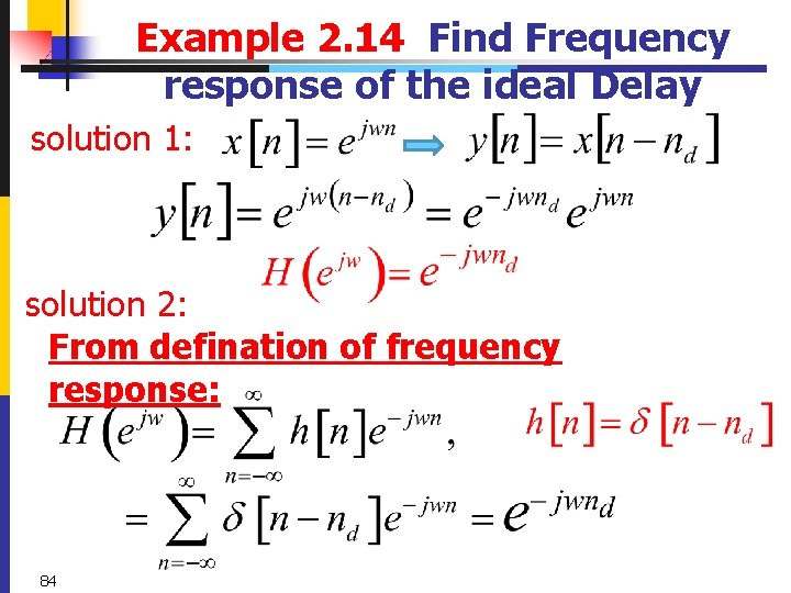
Example 2. 14 Find Frequency response of the ideal Delay solution 1: solution 2: From defination of frequency response: 84

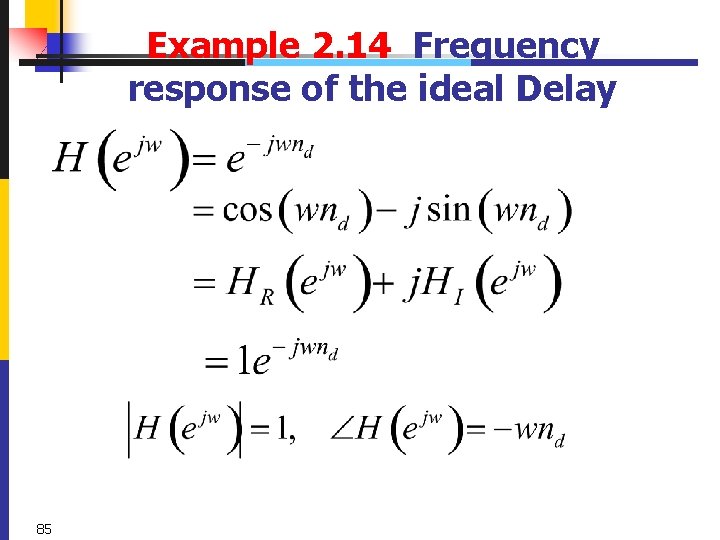
Example 2. 14 Frequency response of the ideal Delay 85

x[n]: Linear combination of complex exponential If , output of LTI system? From the principle of superposition, and the corresponding output of an LTI system is 86

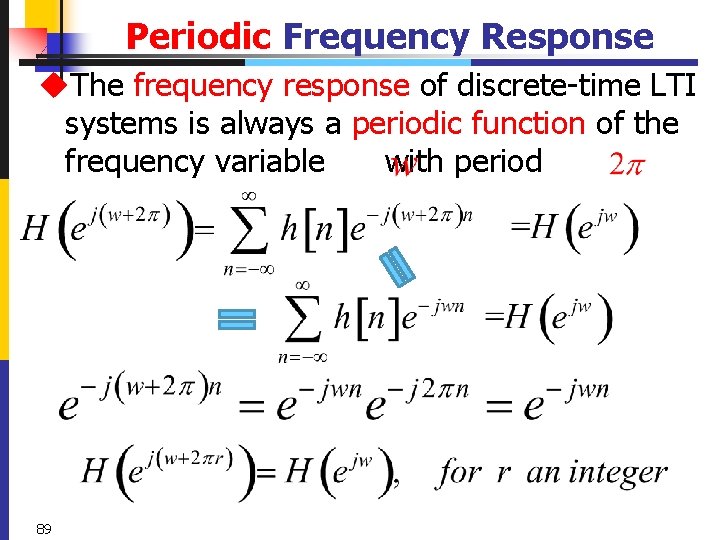
Periodic Frequency Response u. The frequency response of discrete-time LTI systems is always a periodic function of the frequency variable with period 89

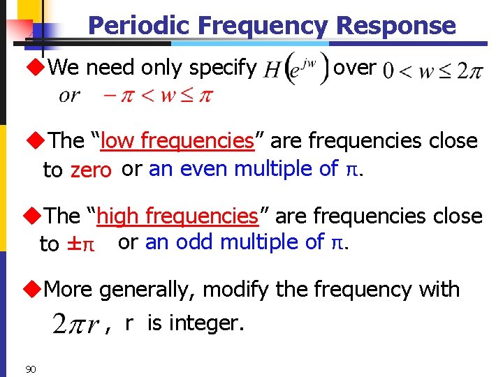
Periodic Frequency Response u. We need only specify over u. The “low frequencies” are frequencies close to zero or an even multiple of π. u. The “high frequencies” are frequencies close to ±π or an odd multiple of π. u. More generally, modify the frequency with , r is integer. 90

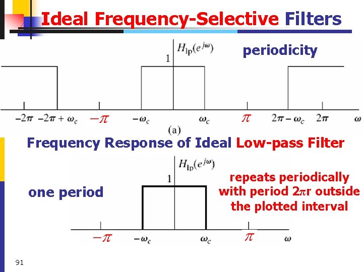
Ideal Frequency-Selective Filters periodicity Frequency Response of Ideal Low-pass Filter one period 91 repeats periodically with period 2πr outside the plotted interval

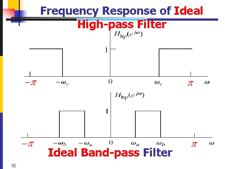
Frequency Response of Ideal High-pass Filter Ideal Band-pass Filter 92

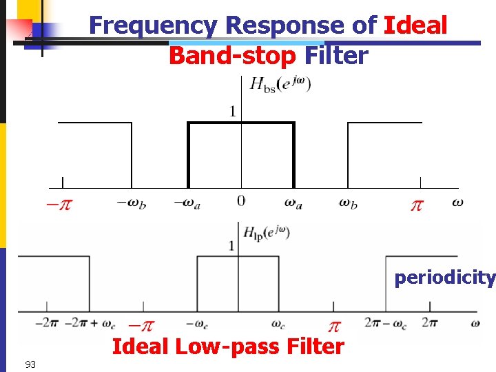
Frequency Response of Ideal Band-stop Filter periodicity 93 Ideal Low-pass Filter

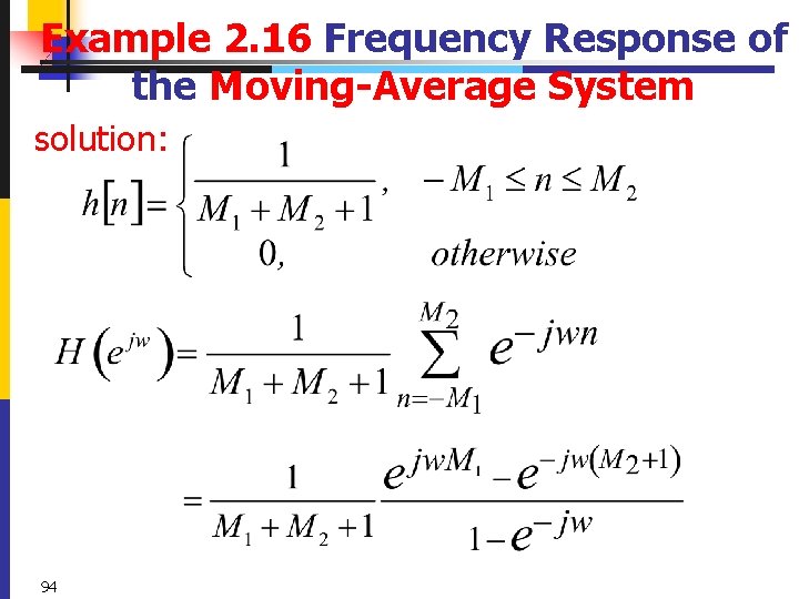
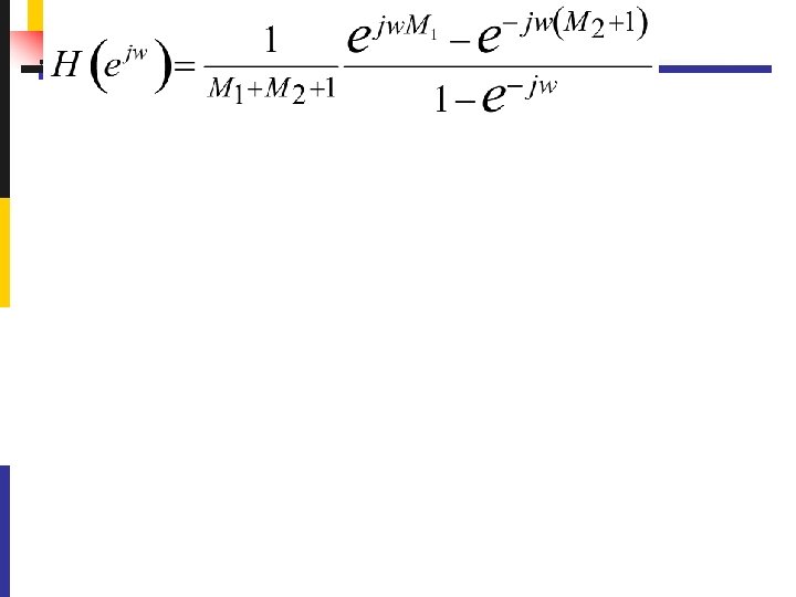
Example 2. 16 Frequency Response of the Moving-Average System solution: 94

95

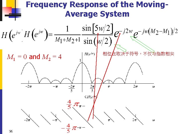
Frequency Response of the Moving. Average System M 1 = 0 and M 2 = 4 96 相位也取决于符号，不仅与指数相关

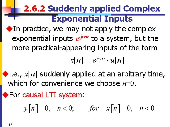
2. 6. 2 Suddenly applied Complex Exponential Inputs u. In practice, we may not apply the complex exponential inputs e jwn to a system, but the more practical-appearing inputs of the form x[n] = ejwn u[n] ui. e. , x[n] suddenly applied at an arbitrary time, which for convenience we choose n=0. u. For causal LTI system: 97

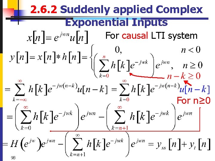
2. 6. 2 Suddenly applied Complex Exponential Inputs For causal LTI system For n≥ 0 98

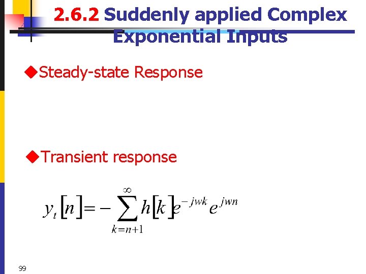
2. 6. 2 Suddenly applied Complex Exponential Inputs u. Steady-state Response u. Transient response 99

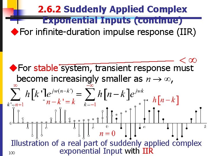
2. 6. 2 Suddenly Applied Complex Exponential Inputs (continue) u. For infinite-duration impulse response (IIR) u. For stable system, transient response must become increasingly smaller as n , Illustration of a real part of suddenly applied complex exponential Input with IIR 100

2. 6. 2 Suddenly Applied Complex Exponential Inputs (continue) u. If h[n] = 0 except for 0 n M (FIR), then the transient response yt[n] = 0 for n+1 > M. Ø For n M, only the steady-state response exists Illustration of a real part of suddenly applied complex exponential Input with FIR 101

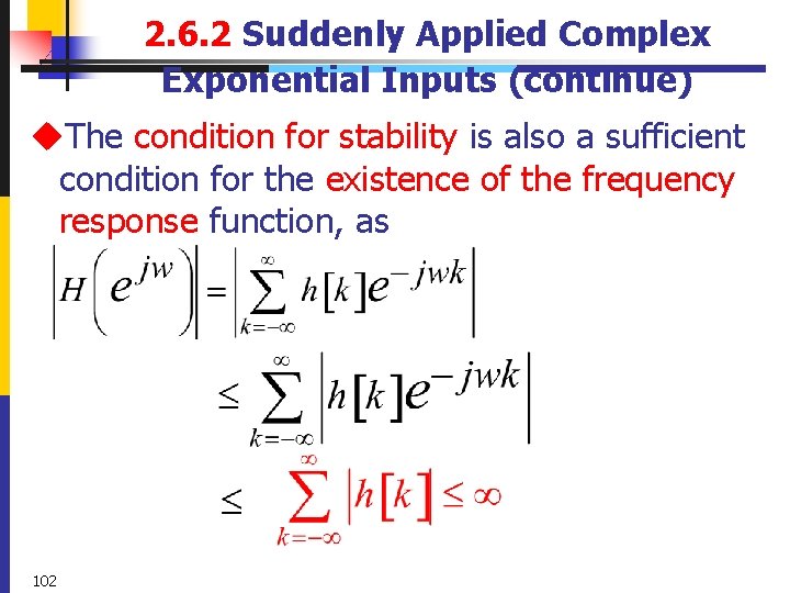
2. 6. 2 Suddenly Applied Complex Exponential Inputs (continue) u. The condition for stability is also a sufficient condition for the existence of the frequency response function, as 102

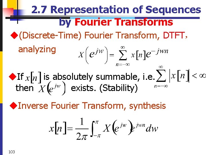
2. 7 Representation of Sequences by Fourier Transforms u(Discrete-Time) Fourier Transform, DTFT， analyzing u. If then is absolutely summable, i. e. exists. (Stability) u. Inverse Fourier Transform, synthesis 103

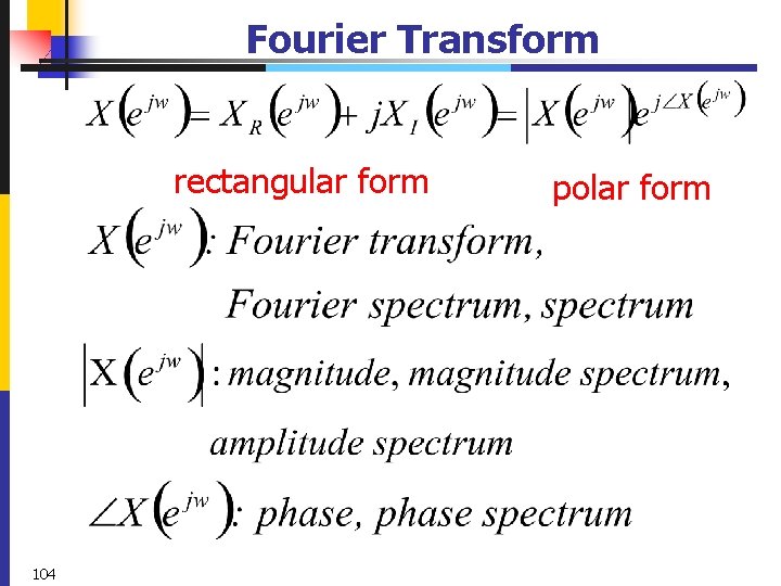
Fourier Transform rectangular form 104 polar form

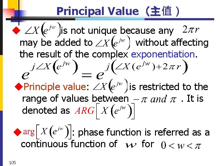
Principal Value（主值） u is not unique because any may be added to without affecting the result of the complex exponentiation. u. Principle value: is restricted to the range of values between. It is denoted as u : phase function is referred as a continuous function of for 105

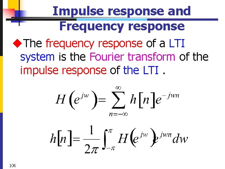
Impulse response and Frequency response u. The frequency response of a LTI system is the Fourier transform of the impulse response of the LTI. 106

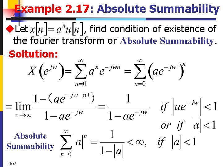
Example 2. 17: Absolute Summability u. Let , find condition of existence of the fourier transform or Absolute Summability. Soltution: Absolute Summability 107

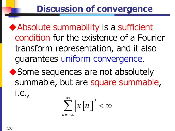
Discussion of convergence u. Absolute summability is a sufficient condition for the existence of a Fourier transform representation, and it also guarantees uniform convergence. u. Some sequences are not absolutely summable, but are square summable, i. e. , 108

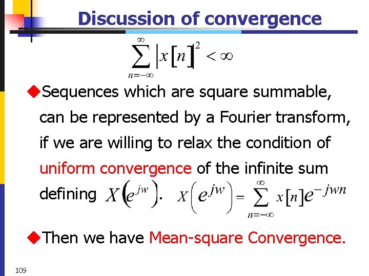
Discussion of convergence u. Sequences which are square summable, can be represented by a Fourier transform, if we are willing to relax the condition of uniform convergence of the infinite sum defining . u. Then we have Mean-square Convergence. 109

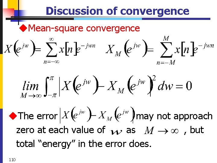
Discussion of convergence u. Mean-square convergence u. The error may not approach zero at each value of as , but total “energy” in the error does. 110

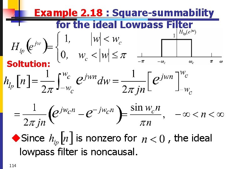
Example 2. 18 : Square-summability for the ideal Lowpass Filter Soltution: u. Since is nonzero for lowpass filter is noncausal. 114 , the ideal

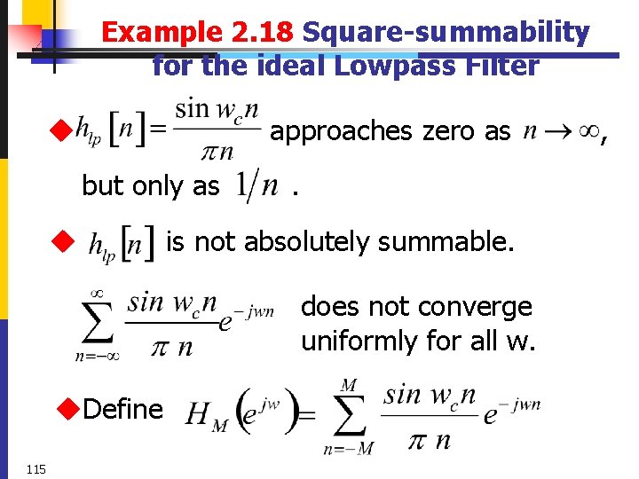
Example 2. 18 Square-summability for the ideal Lowpass Filter approaches zero as u but only as u . is not absolutely summable. does not converge uniformly for all w. u. Define 115 ,

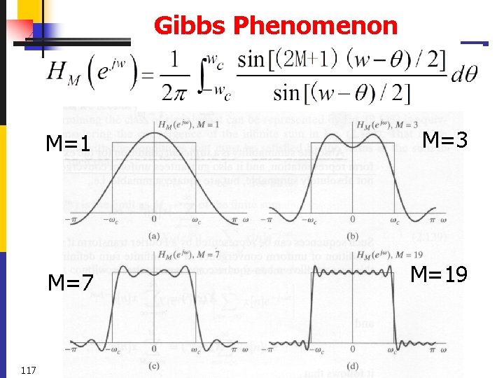
Gibbs Phenomenon 117 M=1 M=3 M=7 M=19

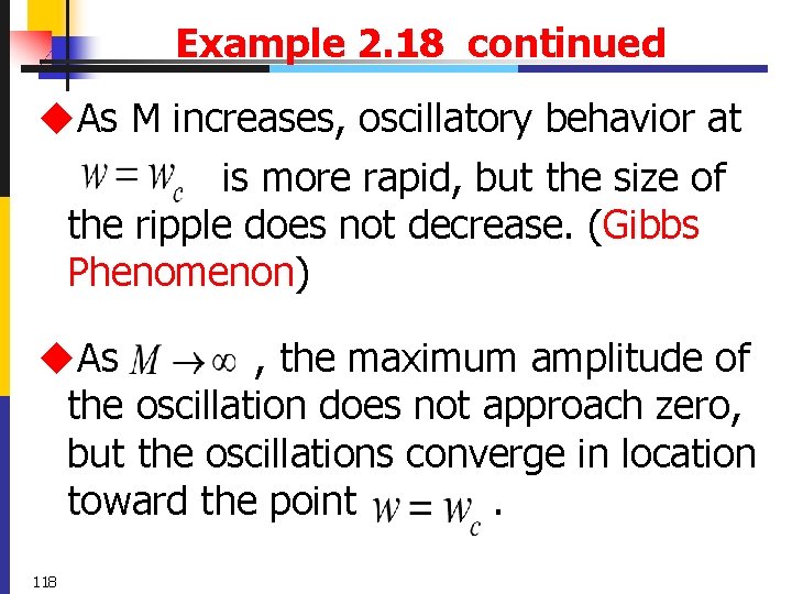
Example 2. 18 continued u. As M increases, oscillatory behavior at is more rapid, but the size of the ripple does not decrease. (Gibbs Phenomenon) u. As , the maximum amplitude of the oscillation does not approach zero, but the oscillations converge in location toward the point. 118

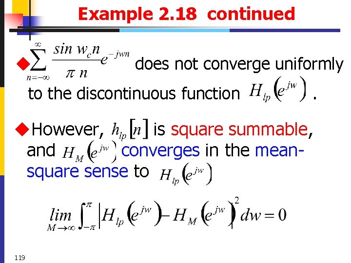
Example 2. 18 continued u does not converge uniformly to the discontinuous function . u. However, is square summable, and converges in the meansquare sense to 119

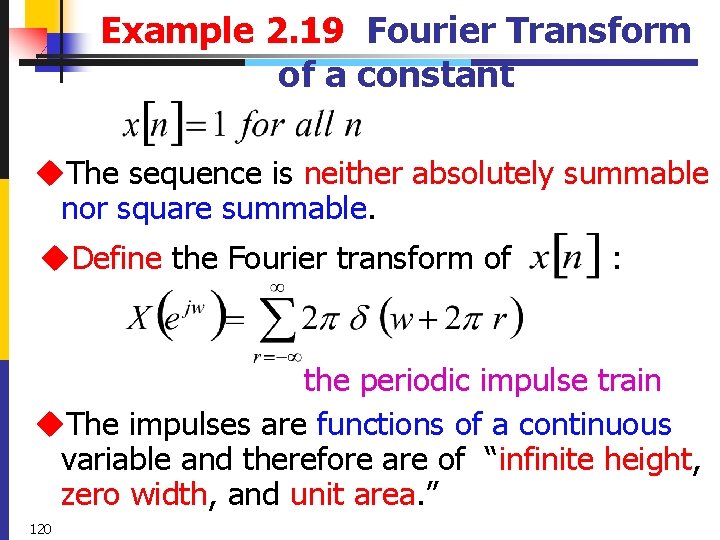
Example 2. 19 Fourier Transform of a constant u. The sequence is neither absolutely summable nor square summable. u. Define the Fourier transform of : the periodic impulse train u. The impulses are functions of a continuous variable and therefore are of “infinite height, zero width, and unit area. ” 120

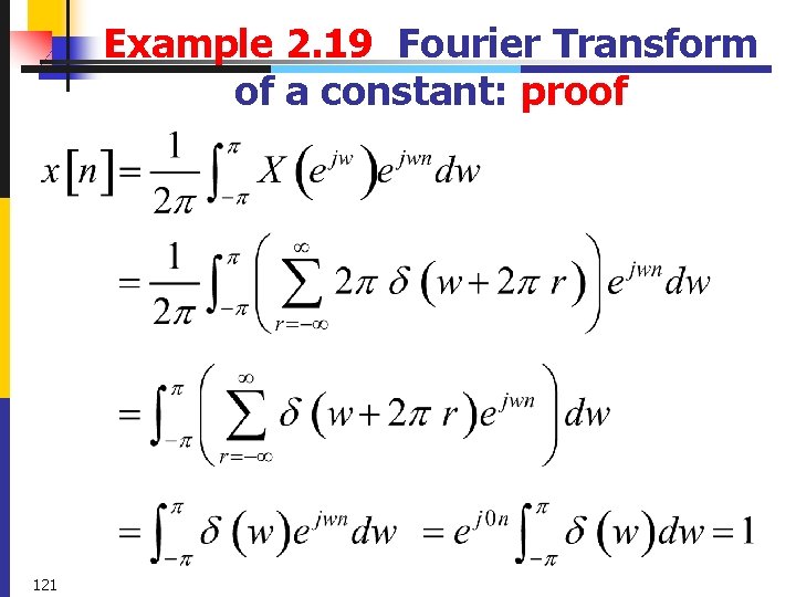
Example 2. 19 Fourier Transform of a constant: proof 121

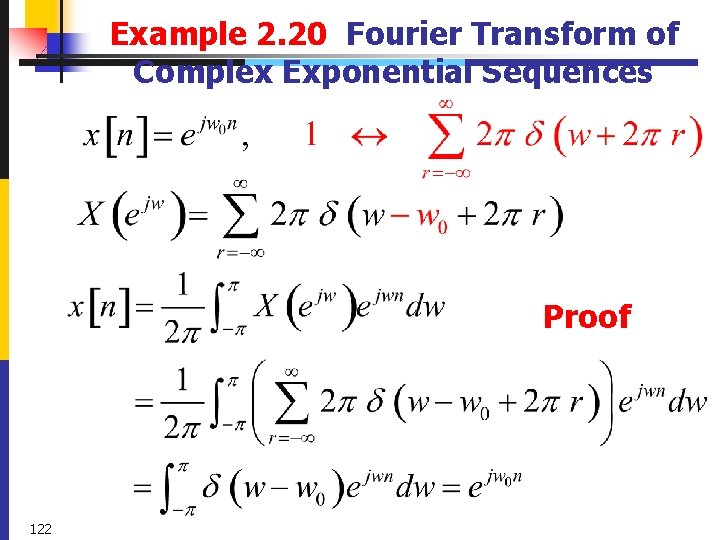
Example 2. 20 Fourier Transform of Complex Exponential Sequences Proof 122

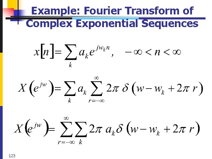
Example: Fourier Transform of Complex Exponential Sequences 123

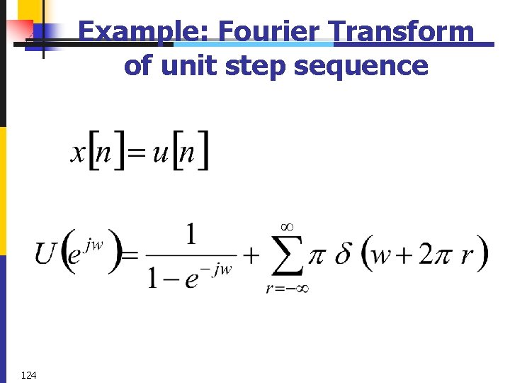
Example: Fourier Transform of unit step sequence 124

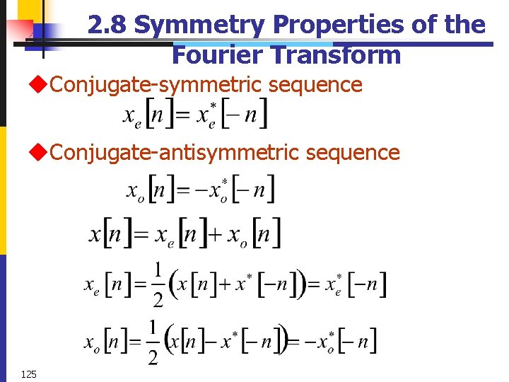
2. 8 Symmetry Properties of the Fourier Transform u. Conjugate-symmetric sequence u. Conjugate-antisymmetric sequence 125

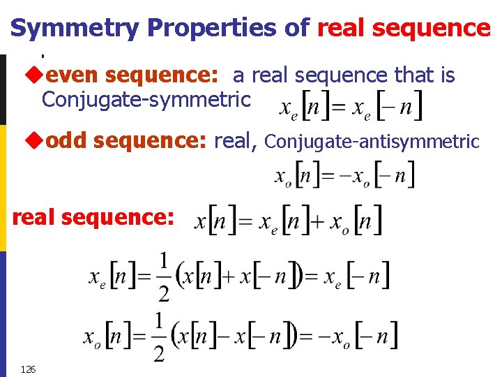
Symmetry Properties of real sequence ueven sequence: a real sequence that is Conjugate-symmetric uodd sequence: real, Conjugate-antisymmetric real sequence: 126

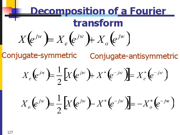
Decomposition of a Fourier transform Conjugate-symmetric 127 Conjugate-antisymmetric

x[n] is complex 128

x[n] is real, Conjugate-symmetric the real part is even, the imaginary part is odd. 129

Ex. 2. 21 illustration of Symmetry Properties x[n] , a is real 130

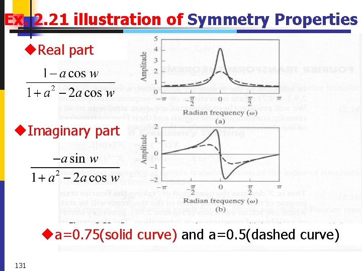
Ex. 2. 21 illustration of Symmetry Properties u. Real part u. Imaginary part ua=0. 75(solid curve) and a=0. 5(dashed curve) 131

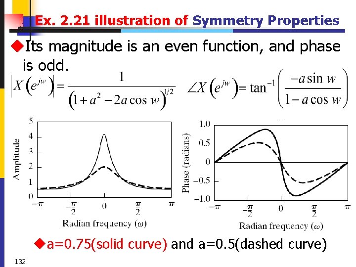
Ex. 2. 21 illustration of Symmetry Properties u. Its magnitude is an even function, and phase is odd. ua=0. 75(solid curve) and a=0. 5(dashed curve) 132

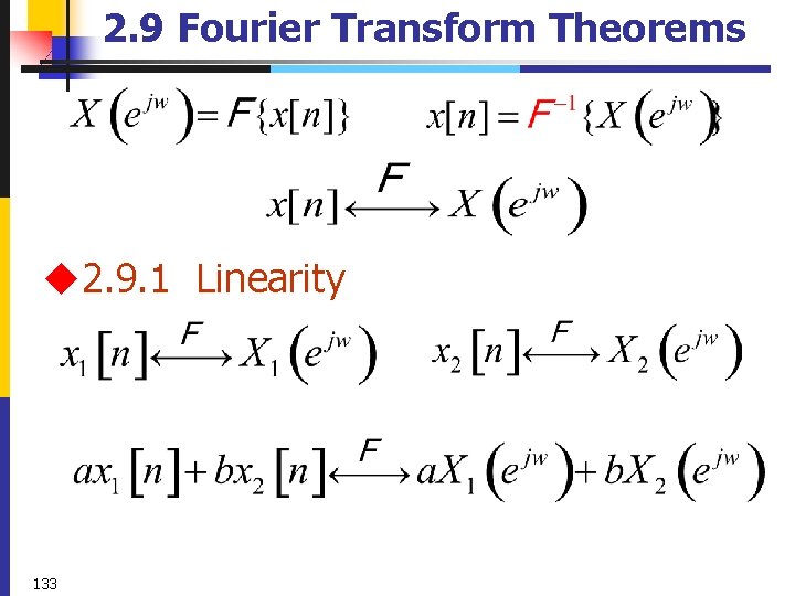
2. 9 Fourier Transform Theorems u 2. 9. 1 Linearity 133

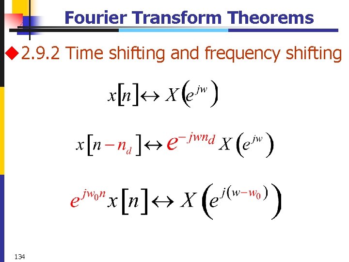
Fourier Transform Theorems u 2. 9. 2 Time shifting and frequency shifting 134

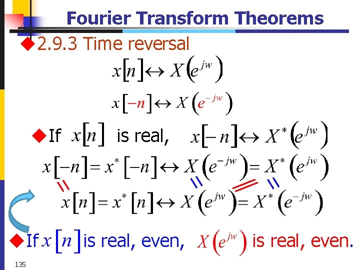
Fourier Transform Theorems u 2. 9. 3 Time reversal u. If 135 is real, even, is real, even.

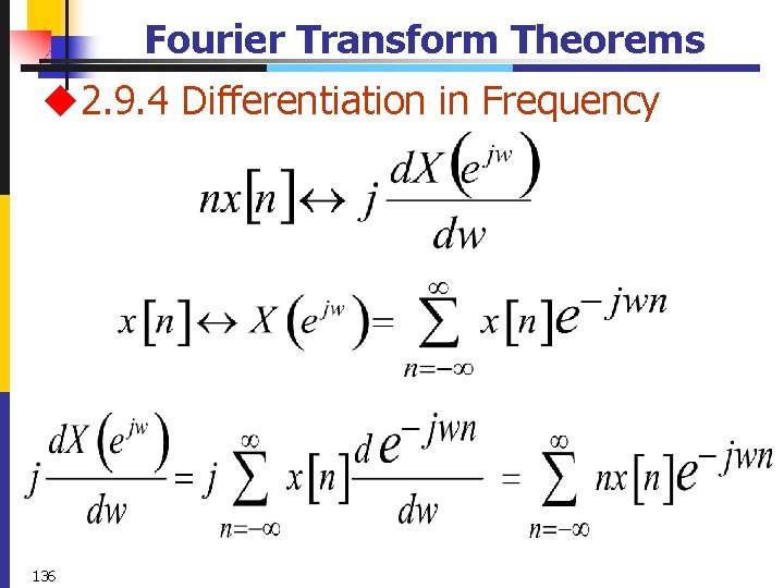
Fourier Transform Theorems u 2. 9. 4 Differentiation in Frequency 136

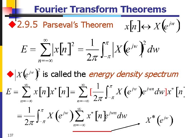
Fourier Transform Theorems u 2. 9. 5 Parseval’s Theorem u 137 is called the energy density spectrum

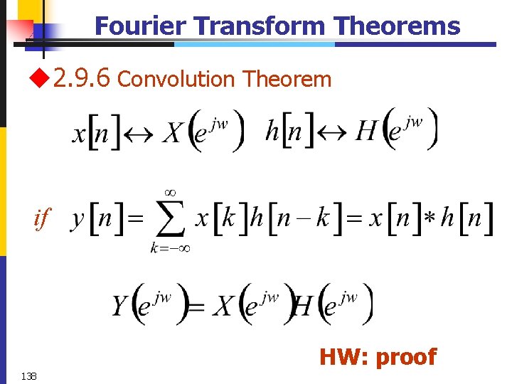
Fourier Transform Theorems u 2. 9. 6 Convolution Theorem if 138 HW: proof

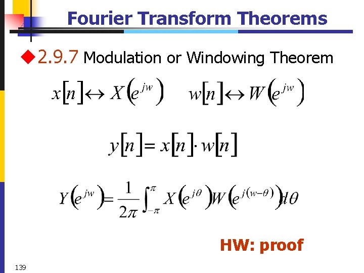
Fourier Transform Theorems u 2. 9. 7 Modulation or Windowing Theorem HW: proof 139

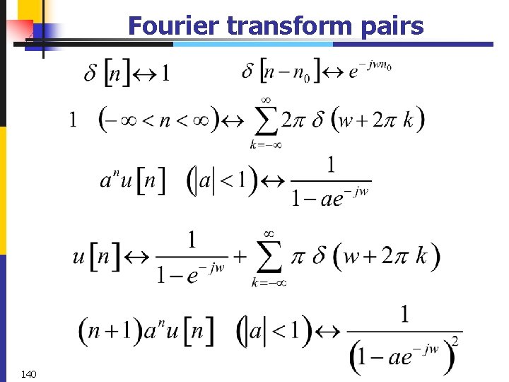
Fourier transform pairs 140

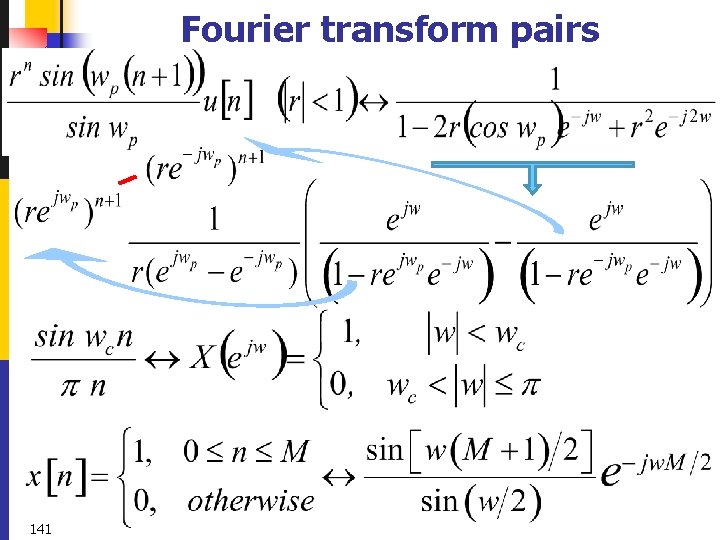
Fourier transform pairs 141

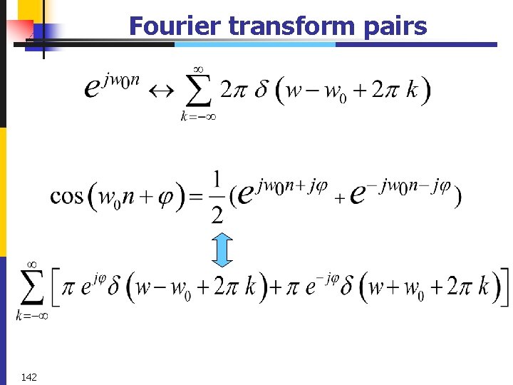
Fourier transform pairs 142

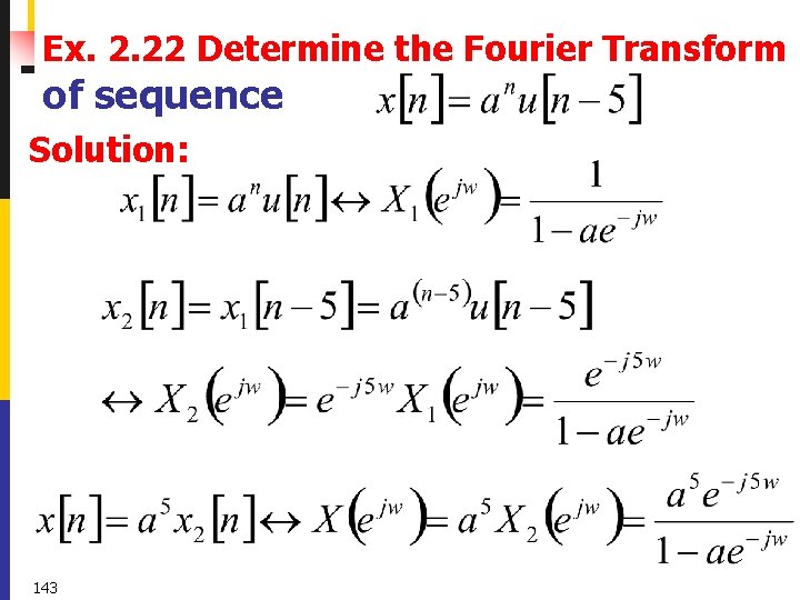
Ex. 2. 22 Determine the Fourier Transform of sequence Solution: 143

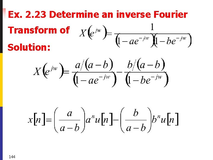
Ex. 2. 23 Determine an inverse Fourier Transform of Solution: 144

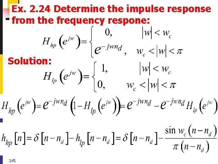
Ex. 2. 24 Determine the impulse response from the frequency respone: Solution: 145

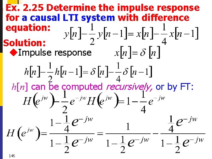
Ex. 2. 25 Determine the impulse response for a causal LTI system with difference equation: Solution: u. Impulse response h[n] can be computed recursively, or by FT: 146

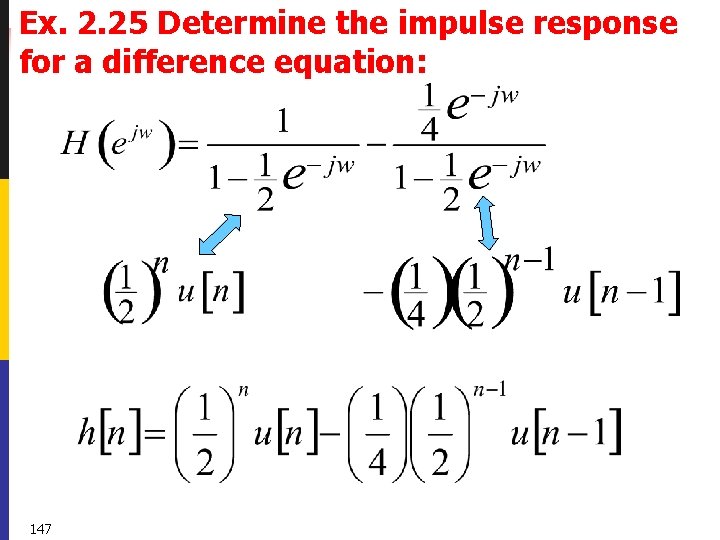
Ex. 2. 25 Determine the impulse response for a difference equation: 147

2. 10 Discrete-Time Random Signals u. Deterministic: each value of a sequence is uniquely determined by a mathematically expression, a table of data, or a rule of some type. u. Stochastic signal: a member of an ensemble of discrete-time signals that is characterized by a set of probability density function. 148

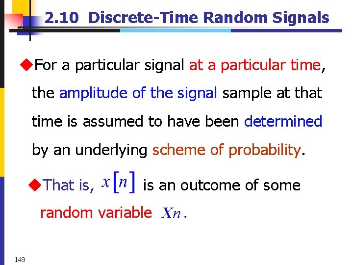
2. 10 Discrete-Time Random Signals u. For a particular signal at a particular time, the amplitude of the signal sample at that time is assumed to have been determined by an underlying scheme of probability. u. That is, is an outcome of some random variable Xn. 149

2. 10 Discrete-Time Random Signals ux[n] is an outcome of some random variable Xn (no necessary to distinguish x[n] and Xn ). u. The collection of random variables is called a random process(随机过程). u The stochastic signals do not directly have Fourier transform, but the Fourier transform of the autocorrelation and autocovariance sequece often exist. 150

Fourier transform in stochastic signals u. The Fourier transform of autocorrelation sequence has a useful interpretation in terms of the frequency distribution of the power in the signal. u. The effect of processing stochastic signals with a discrete-time LTI system can be described in terms of the effect of the system on the autocorrelation sequence. 151

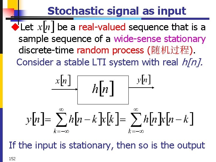
Stochastic signal as input u. Let be a real-valued sequence that is a sample sequence of a wide-sense stationary discrete-time random process (随机过程). Consider a stable LTI system with real h[n]. If the input is stationary, then so is the output 152

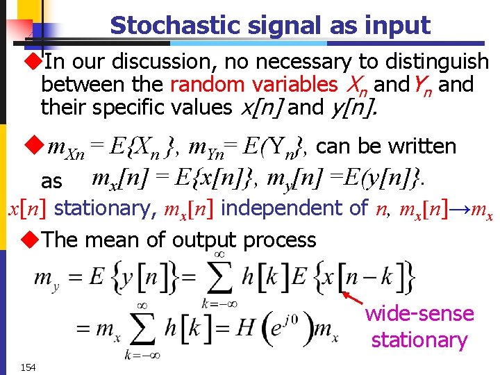
Stochastic signal as input u. In our discussion, no necessary to distinguish between the random variables Xn and. Yn and their specific values x[n] and y[n]. um. Xn = E{Xn }, m. Yn= E(Yn}, can be written as mx[n] = E{x[n]}, my[n] =E(y[n]}. x[n] stationary, mx[n] independent of n, mx[n]→mx u. The mean of output process wide-sense stationary 154

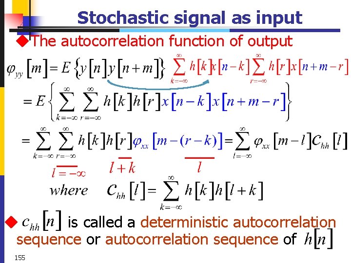
Stochastic signal as input u. The autocorrelation function of output u is called a deterministic autocorrelation sequence or autocorrelation sequence of 155

Stochastic signal as input real h[n] power (density) spectrum DTFT of the autocorrelation function of output 156

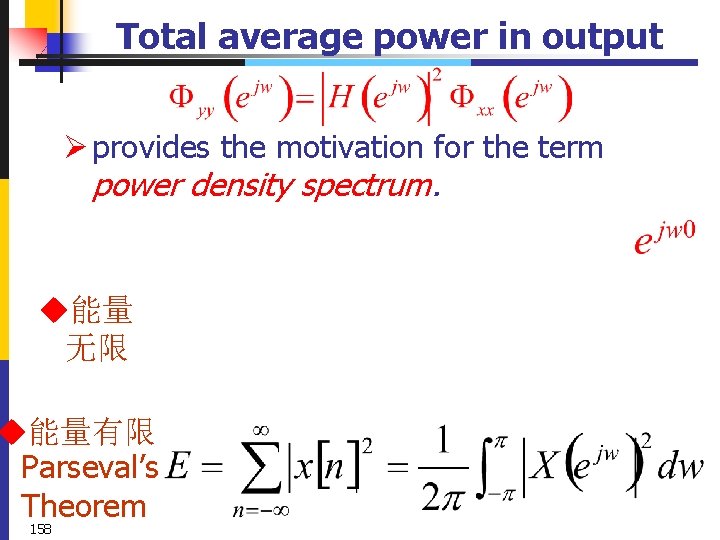
Total average power in output Ø provides the motivation for the term power density spectrum. u能量 无限 u能量有限 Parseval’s Theorem 158

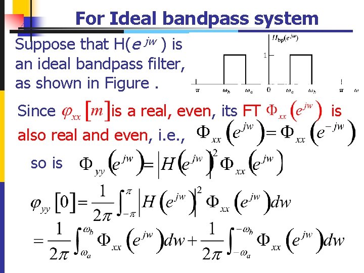
For Ideal bandpass system Suppose that H(e jw ) is an ideal bandpass filter, as shown in Figure. Since is a real, even, its FT also real and even, i. e. , so is is

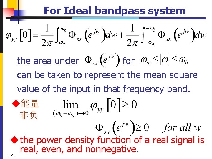
For Ideal bandpass system the area under for can be taken to represent the mean square value of the input in that frequency band. u能量 非负 u the power density function of a real signal is real, even, and nonnegative. 160

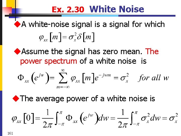
Ex. 2. 30 White Noise u. A white-noise signal is a signal for which u. Assume the signal has zero mean. The power spectrum of a white noise is u. The average power of a white noise is 161

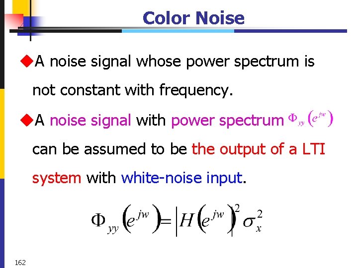
Color Noise u. A noise signal whose power spectrum is not constant with frequency. u. A noise signal with power spectrum can be assumed to be the output of a LTI system with white-noise input. 162

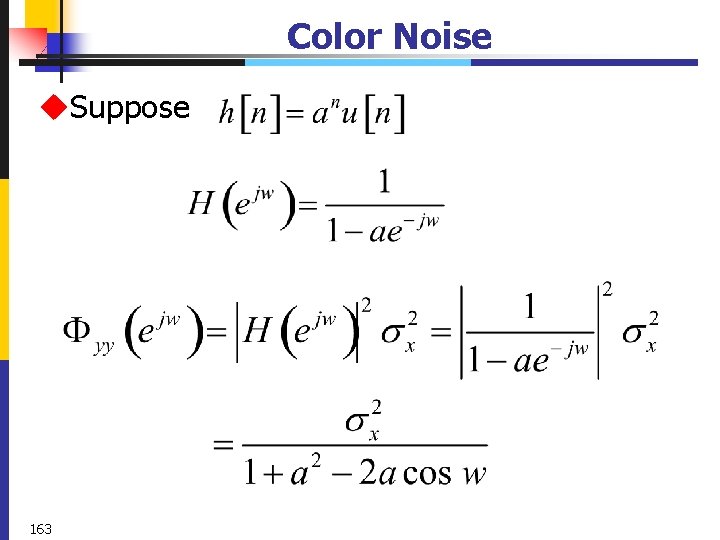
Color Noise u. Suppose 163

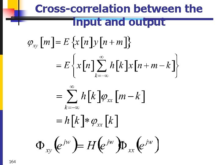
Cross-correlation between the input and output 164

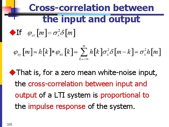
Cross-correlation between the input and output u. If u. That is, for a zero mean white-noise input, the cross-correlation between input and output of a LTI system is proportional to the impulse response of the system. 165

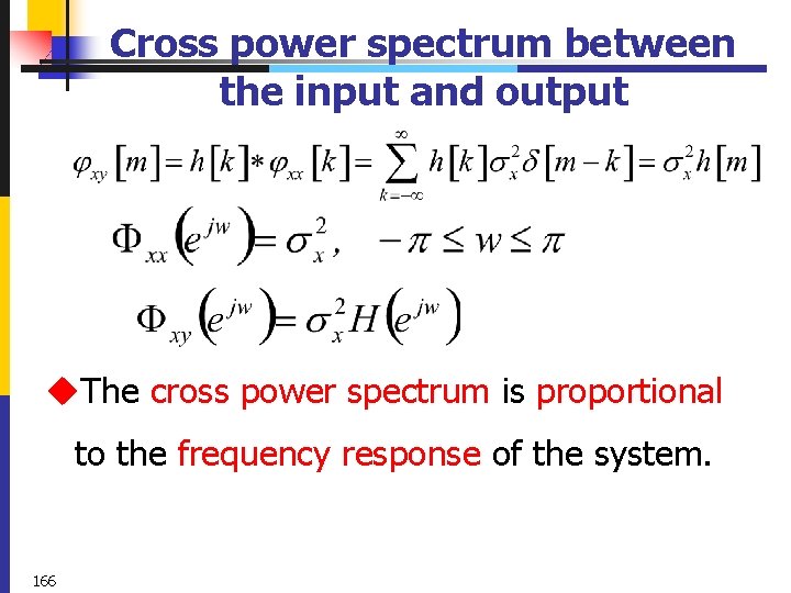
Cross power spectrum between the input and output u. The cross power spectrum is proportional to the frequency response of the system. 166

2. 11 Summary u. Define a set of basic sequence. u. Define and represent the LTI systems in terms of the convolution, stability and causality. u. Introduce the linear constant-coefficient difference equation with initial rest conditions for LTI , causal system. u. Recursive solution of linear constantcoefficient difference equations. 167

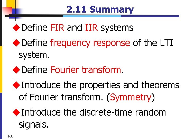
2. 11 Summary u. Define FIR and IIR systems u. Define frequency response of the LTI system. u. Define Fourier transform. u. Introduce the properties and theorems of Fourier transform. (Symmetry) u. Introduce the discrete-time random signals. 168

Chapter 2 HW u 2. 4, 2. 5, 2. 11, 2. 20 u 2. 2, 2. 5, 2. 7, 2. 12, 2. 62 169 返 回 2021/12/18 上一页 Zhongguo Liu_Biomedical Engineering_Shandong Univ. 下一页