Biologically Inspired Computing Finishing off EC and incorporating

Biologically Inspired Computing: Finishing off EC, and incorporating CW 1 This is lecture 5 of `Biologically Inspired Computing’ Contents: Steady state and generational EAs, basic ingredients, example run-throughs on the TSP, example encodings, hillclimbing, landscapes

Four topics • Hillclimbing and Local search (motivating EAs via problems with simpler methods, rather than via natural Evolution) • Landscapes • Neighbourhoods • Encodings

Simplest possible EA: Hillclimbing 0. Initialise: Generate a random solution c; evaluate its fitness, f(c). Call c the current solution. 1. Mutate a copy of the current solution – call the mutant m Evaluate fitness of m, f(m). 2. If f(m) is no worse than f(c), then replace c with m, otherwise do nothing (effectively discarding m). 3. If a termination condition has been reached, stop. Otherwise, go to 1. Note. No population (well, population of 1). This is a very simple version of an EA, although it has been around for much longer.

Example on a 1 D landscape 200 0 0 10 20 30 40 FITNESS -200 -400 -600 -800 -1000 -1200 -1400 -1600 -1800 x - the ‘genotype’ 50 60

Initial random point 200 0 0 10 20 30 40 FITNESS -200 -400 -600 -800 -1000 -1200 -1400 -1600 -1800 x - the ‘genotype’ 50 60

mutant 200 0 0 10 20 30 40 FITNESS -200 -400 -600 -800 -1000 -1200 -1400 -1600 -1800 x - the ‘genotype’ 50 60
 200 0 0 10 20 30 40 FITNESS -200 -400 -600")
Current solution (unchanged) 200 0 0 10 20 30 40 FITNESS -200 -400 -600 -800 -1000 -1200 -1400 -1600 -1800 x - the ‘genotype’ 50 60

Next mutant 200 0 0 10 20 30 40 FITNESS -200 -400 -600 -800 -1000 -1200 -1400 -1600 -1800 x - the ‘genotype’ 50 60

New current solution 200 0 0 10 20 30 40 FITNESS -200 -400 -600 -800 -1000 -1200 -1400 -1600 -1800 x - the ‘genotype’ 50 60

Next mutant 200 0 0 10 20 30 40 FITNESS -200 -400 -600 -800 -1000 -1200 -1400 -1600 -1800 x - the ‘genotype’ 50 60

New current solution 200 0 0 10 20 30 40 FITNESS -200 -400 -600 -800 -1000 -1200 -1400 -1600 -1800 x - the ‘genotype’ 50 60

ETC …………… 200 0 0 10 20 30 40 FITNESS -200 -400 -600 -800 -1000 -1200 -1400 -1600 -1800 x - the ‘genotype’ 50 60

How will HC do on this landscape? 2 1 0 0 -1 -2 -3 -4 -5 -6 -7 -8 10 20 30 40 50 60

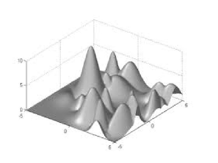
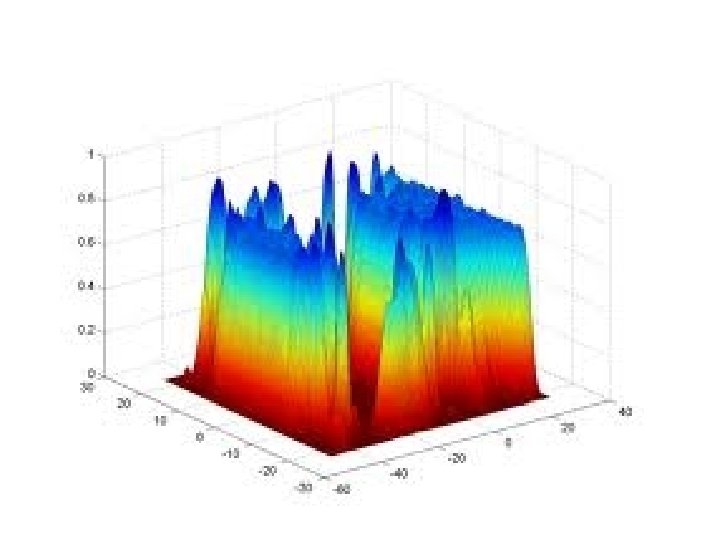
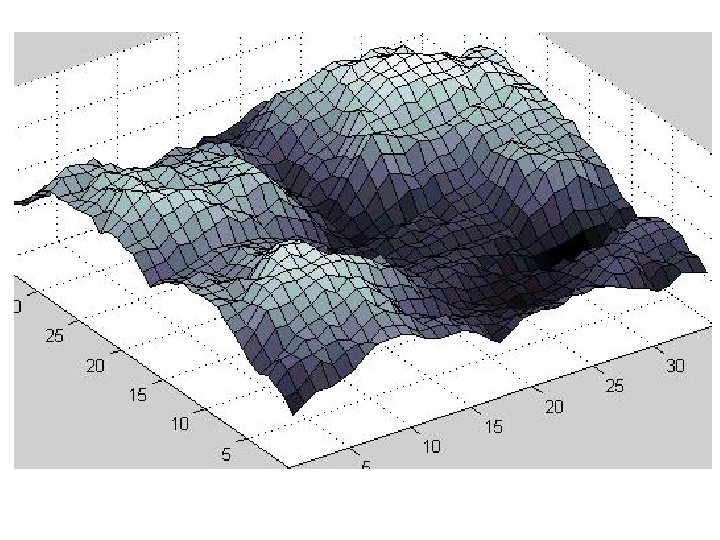
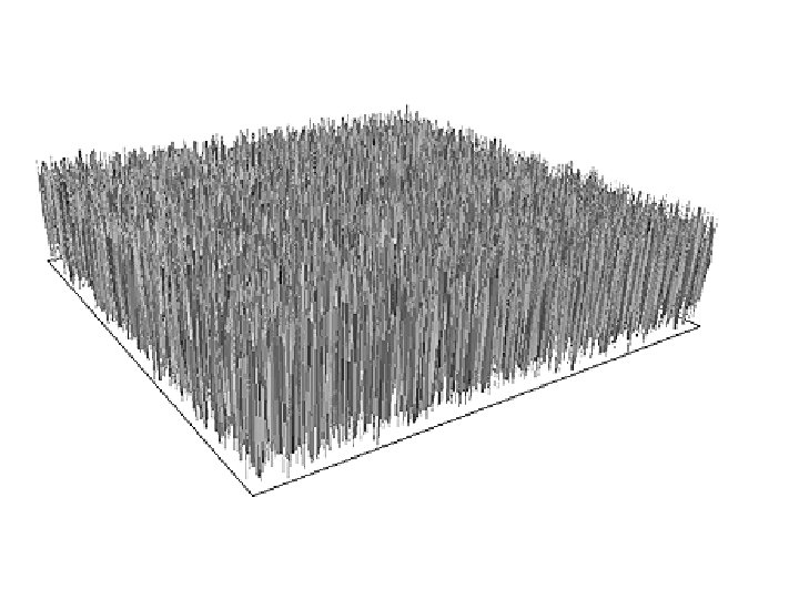
Some other landscapes
, the fitness of a candidate in")
Landscapes Recall S, the search space, and f(s), the fitness of a candidate in S f(s) members of S lined up along here The structure we get by imposing f(s) on S is called a landscape
, the fitness of a candidate in")
Neighbourhoods Recall S, the search space, and f(s), the fitness of a candidate in S f(s) 0 1 2 3 4 5 6 7 8 9 10 11 12 13 14 15 16 17 Showing the neighbourhoods of two candidate solutions, assuming The mutation operator adds a random number between − 1 and 1
, the fitness of a candidate in")
Neighbourhoods Recall S, the search space, and f(s), the fitness of a candidate in S f(s) 0 1 2 3 4 5 6 7 8 9 10 11 12 13 14 15 16 17 Showing the neighbourhood of a candidate solutions, assuming The mutation operator adds a random integer between − 2 and 2
, the fitness of a candidate in")
Neighbourhoods Recall S, the search space, and f(s), the fitness of a candidate in S f(s) 0 1 2 3 4 5 6 7 8 9 10 11 12 13 14 15 16 17 Showing the neighbourhood of a candidate solutions, assuming the mutation operator simply changes the solution to a new random Number between 0 and 20
, the fitness of a candidate in")
Neighbourhoods Recall S, the search space, and f(s), the fitness of a candidate in S f(s) 0 1 2 3 4 5 6 7 8 9 10 11 12 13 14 15 16 17 Showing the neighbourhood of a candidate solution, assuming the mutation operator adds a Gaussian (ish) with mean zero.
 is our fitness function, and")
Neighbourhoods Let s be an individual in S, f(s) is our fitness function, and M is our mutation operator, so that M(s 1) s 2, where s 2 is a mutant of s 1. Given M, we can usually work out the neighbourhood of an individual point s – the neighbourhood of s is the set of all possible mutants of s E. g. Encoding: permutations of k objects (e. g. for k-city TSP) Mutation: swap any adjacent pair of objects. Neighbourhood: Each individual has k neighbours. E. g. neighbours of EABDC are: {AEBDC, EBADC, EADBC, EABCD, CABDE} Encoding: binary strings of length L (e. g. for L-item bin-packing) Mutation: choose a bit randomly and flip it. Neighbourhood: Each individual has L neighbours. E. g. neighbours of 00110 are: {10110, 01110, 00010, 00100, 00111}

Landscape Topology Mutation operators lead to slight changes in the solution, which tend to lead to slight changes in fitness. Why are “big mutations” generally a bad idea to have in a search algorithm ? ?
 members of S lined up along here Typically, with large (realistic)")
Typical Landscapes f(s) members of S lined up along here Typically, with large (realistic) problems, the huge majority of the landscape has very poor fitness – there are tiny areas where the decent solutions lurk. So, big random changes are very likely to take us outside the nice areas.

Typical Landscapes Unimodal Multimodal Plateau Deceptive As we home in on the good areas, we can identify broad types of Landscape feature. Most landscapes of interest are predominantly multimodal. Despite being locally smooth, they are globally rugged

Beyond Hillclimbing HC clearly has problems with typical landscapes: There are two broad ways to improve HC, from the algorithm viewpoint: 1. Allow downhill moves – a family of methods called Local Search does this in various ways. 2. Have a population – so that different regions can be explored inherently in parallel – I. e. we keep `poor’ solutions around and give them a chance to `develop’.
 = b;")
Local Search Initialise: Generate a random solution c; evaluate its fitness, f(s) = b; call c the current solution, and call b the best so far. Repeat until termination conditon reached: 1. Search the neighbourhood of c, and choose one, m Evaluate fitness of m, call that x. 2. According to some policy, maybe replace c with x, and update c and b as appropriate. E. g. Monte Carlo search: 1. same as hillclimbing; 2. If x is better, accept it as new current solution; if x is worse, accept it with some probabilty (e. g. 0. 1). E. g. tabu search: 1. evaluate all immediate neighbours of c 2. choose the best from (1) to be the next current solution, unless it is `tabu’ (recently visited), in which choose the next best, etc.

Population-Based Search • Local search is fine, but tends to get stuck in local optima, less so than HC, but it still gets stuck. • In PBS, we no longer have a single `current solution’, we now have a population of them. This leads directly to the two main algorithmic differences between PBS and LS – Which of the set of current solutions do we mutate? We need a selection method – With more than one solution available, we needn’t just mutate, we can [mate, recombine, crossover, etc …] two or more current solutions. • So this is an alternative route towards motivating our nature-inspired EAs – and also starts to explain why they turn out to be so good.
 Direct vs Indirect")
Encodings (aka representation) Direct vs Indirect
 EC Note that: • Given")
Encoding / Representation Maybe the main issue in (applying) EC Note that: • Given an optimisation problem to solve, we need to find a way of encoding candidate solutions • There can be many very different encodings for the same problem • Each way affects the shape of the landscape and the choice of best strategy for climbing that landscape.

E. g. encoding a timetable I 9: 00 4, 5, 13, 1, 1, 7, 13, 2 mon tue E 4, E 5 E 2 wed thur E 3, E 7 11: 00 E 8 2: 00 E 6 4: 00 E 1 Exam 2 in 5 th slot Exam 1 in 4 th slot Etc … • Generate any string of 8 numbers between 1 and 16, and we have a timetable! • Fitness may be <clashes> + <consecs> + etc … • Figure out an encoding, and a fitness function, and you can try to evolve solutions.

Mutating a Timetable with Encoding 1 9: 00 4, 5, 13, 1, 1, 7, 13, 2 mon tue E 4, E 5 E 2 11: 00 E 8 2: 00 4: 00 E 6 E 1 Using straightforward single-gene mutation Choose a random gene wed thur E 3, E 7

Mutating a Timetable with Encoding 1 mon tue E 4, E 5 E 2 11: 00 E 8 E 3 2: 00 E 6 9: 00 4, 5, 6 , 1, 1, 7, 13, 2 4: 00 E 1 Using straightforward single-gene mutation One mutation changes position of one exam wed thur E 7

Alternative ways to do it This is called a `direct’ encoding. Note that: • A random timetable is likely to have lots of clashes. • The EA is likely (? ) to spend most of its time crawling through clash-ridden areas of the search space. • Is there a better way?

E. g. encoding a timetable II mon 9: 00 4, 5, 13, 1, 1, 7, 13, 2 tue E 4, E 5 wed thur E 3, E 7 11: 00 E 8 2: 00 4: 00 E 6, E 2 E 1 Etc … Use the 13 th clash-free slot for exam 3 Use the 5 th clash-free slot for exam 2 (clashes with E 4, E 8) Use the 4 th clash-free slot for exam 1

So, a common approach is to build an encoding around an algorithm that builds a solution • Don’t encode a candidate solution directly E 2 • … instead encode parameters/features for a constructive algorithm that builds a candidate solution

e. g. : bin-packing – given collection of items, pack them into the fewest possible number of bins

e. g. : bin-packing – given collection of items, pack them into the fewest possible number of bins

Engineering Constructive Algorithms A typical constructive algorithm for bin-packing: Put the items in a specific sequence (e. g. smallest to largest) Initialise solution Repeat nitems times choose next item, place it in first bin it fits (create a new empty bin if necessary) Indirect Encodings often involve using a constructive algorithm,
 constructive algorithm for bin-packing FFA")
Example using ‘First-Fit Ascending’ (FFA) constructive algorithm for bin-packing FFA

First-fit Ascending

First-fit Ascending

First-fit Ascending

First-fit Ascending

First-fit Ascending

First-fit Ascending

Example using First-Fit Descending First-fit Descending

First-Fit Descending

First-Fit Descending

First-Fit Descending

First-Fit Descending

First-Fit Descending

Notes: • In other problems, FFA gets better results than FFD • There are many other constructive heuristics for bin packing, e. g. Using formulae that choose next item based on distribution of unplaced item sizes and empty spaces. . . • There are constructive algorithms for most problems (e. g. Timetabling, scheduling, etc. . ) • Often, ‘indirect encodings’ for EAs use constructive algorithms. • Common approach: the encoding is permutation, and the solution is built using the items in that order • READ THE FALKENAUER PAPER TO SEE GOOD EA ENCODING FOR BIN-PACKING

Other well known constructive algorithms • Prim’s algorithm for building the minimal spanning tree (see an earlier lecture) is an example. • Djikstra’s shortest path algorithm is also an example. • In both of these cases, the optimal solution is guaranteed to be found, since MST and SP are easy problems. • But usually we see constructive methods used to give very fast `OK’ solutions to hard problems.

On engineering constructive methods Some Constructive Heuristics are deterministic. I. e. they give the same answer each time. Some are stochastic – I. e. they may give a different solution in different runs. Usually, if we have a deterministic constructive method such as FFD, we can engineer a stochastic version of it. E. g. instead of choosing the next-lightest item in each step, we might choose randomly between the lightest three unplaced items.

Bin packing example direct encoding: 2, 3, 1. . item 1 is in bin 2, item 2 is in bin 3, item 3 is in bin 2, etc. . . (often a bin will be over capacity, so fitness function will have to include penalties) Bin packing example indirect encoding: candidate solution is a perm of the items, e. g. 4, 2, 1, 3, 5. . . meaning: First place item 4 in the first available bin it fits in, then place item 2 in the first available. . . etc.
 phenotype (actual solution) mapping •")
Direct vs Indirect Encodings Direct: • straightforward genotype (encoding) phenotype (actual solution) mapping • Easy to estimate effects of mutation • Fast interpretation of chromosome (hence speedier fitness evlaluation) Indirect/Hybrid: • Easier to exploit domain knowledge – (e. g. use this in the constructive heuristic) • Hence, possible to `encode away’ undesirable features • Hence, can seriously cut down the size of the search space • But, slow interpretation • Neighbourhoods are highly rugged.
 D 1,")
Example real-number Encoding (and: How EAs can innovate, rather than just optimize) D 1, D 2, D 3, D 4 D 5 D 6 D 1 >= D 2 >= D 3, D 4 <= D 5 <= D 6 Fixed at six diameters, five sections Design shape for a two-phase jet nozzle

A simple encoding 2, 1. 8, 1. 1, 1. 3 The encoding enforces these constraints: D 1 >= D 2 >= D 3, D 4 <= D 5 <= D 6 Fixed at six diameters, five sections 1. 5

A more complex encoding– bigger search space, slower, but potential for innovative solutions Num sections before smallest Z 1, Z 2, Section diameters D 1, D 2, D 3 Dsmall…, Dn+1, … Num sections after smallest Middle section constrained to be smallest, That’s all Mutations can change diameters, add sections, and delete sections

CW 1
, and")
There follow three example slides (of the kind I expect you to submit), and then a description of the coursework.

Example EC Application Scheduling Earth Observing Satellites with Evolutionary Algorithms http: //alglobus. net/NASAwork/papers/SMCIT 03/SMCIT 02 paper 3. pdf An EOS fleet has specific observation & image capture targets and is subject to many constraints. This looks at two cases involving 1 and 2 satellites in fixed orbits Encoding: is a Permutation of Image. Tasks – each is a specific area that must be observed once per day. A ‘scheduler’ routine then determines satellite ‘slews’ and other resources that have to be spent to achieve the requests in this order. Fitness: in these simple cases, fitness was a combination of penalties for (i) unmet Image. Tasks, (ii) total time slweing (ii) sum of slew angles. Hence this measured meeting of target with minimal wear and tear and optimised image quality. Results: HC, SA and EA were compared on these simple cases; SA was found best. Also, they found combined scheduling was better than independent scheduling of each satellite in a fleet

Example EC Application Design of Reinforced Concrete Frames using a Genetic Algorithm http: //www. ce. memphis. edu/pezeshk/PDFs/camp_pezeshk_hakan. pdf Design dimensions and steel reinforcement params for structural beams meeting building constraints Various test case scenarios looked at, including the six storey example on the right, inolving a set of RC elements Encoding: simple list of numbers representing depth and height parameters, and number of placement of steel reinforcement sections. Fitness: calculated with standard equations used by standards bodies Results: They found that a simple GA worked adequately, leading to small reduction in structural costs while remaining safe and legal.

Example EC Application A genetic algorithm for 2 D orthogonal packing http: //www. research. att. com/techdocs/TD_7 M 7 QJG. pdf Specific shapes (e. g. PVC, glass, plywood, . . . ) have to be cut from sheet with minimal waste. E. g. wasteful & optimal solutions shown on right. Tested on many benchmark probs with size ranging from 10— 100 shapes. Paper focuses on new fitness function which considers the empty rectangular spaces, aiming to help direct search towards sols that can be more likely improved by mutation. Encoding: two permutations in each solution: (i) or of shapes (ii) order of plaement procedures – each of these is a choice from a small no. of simple heuristics. E. g. “BL” means close as poss to bottom left. Results: New technique does very well, compared with a wide range of approaches on the same roblems

BIC: Coursework 1 Produce FOUR slides, each briefly describing a different application of evolutionary computation (or another bio-inspired approach) on an optimization problem. The previous three slides are examples of the type of thing I am looking for. EACH SLIDE MUST: (i) contain a URL to a paper, thesis or other source that describes this application (ii) contain at least one graphic/figure (iii) simply and briefly explain key details of the problem, the encoding, the fitness function, and the findings in the paper. HOW MUCH I EXPECT FROM YOU: Use google scholar, or maybe just google, and use sensible and creative search keywords. Don’t go overboard in the time you spend on this – e. g. I did not read in detail the papers summarised in the previous 3 slides. I just tried to grab the key ideas, and make up a slide that simply conveys the gist of them. MARKING: Each of your slides will get 0, 1, 2 or 3 marks. When I have all your slides, I will add a further 0, 1, 2 or 3 marks for the overall level of diversity and interestingness E. g. If they are all about very similar applications, you get 0, although maybe 1 if quite different approaches to encoding or fitness are involved. SEE NEXT SLIDE

BIC: Coursework 1: more about marking and handin To hand in, please email each individual slide in a separate message, as follows: – send it to dwcorne@gmail. com – include the slide (either ppt or pdf) as an attachment –put your (real) name and degree programme (e. g. BSc CS, MSc AI, whatevs) in the body of the email –Make the subject line: “BIC CW 1 Slide N”, where N is either 1, 2, 3 or 4 –Hand in slide 1 before 23: 59 pm YESTERDAY 16 th Oct –Hand in slide 2 before 23: 59 pm Wednesday 30 th Oct –Hand in slide 3 and slide 4 before 23: 59 pm Wednesday 17 th Nov Earlier handins for any slide are fine. Each slide handed in after Wednesday 17 th will result in a 2 marks penalty. E. g. : if your slide marks are 2, 3, 1 and 3, your diversity mark is 2, and you handed in 2 of the slides late, then you will get 7 out of 15

Mandatory additional material Further encodings: Grouping problems, Rules, Trees. EA basics: Selection, Operators
- Slides: 70