BIOInspired Algorithms And Its Application Thomas K P

BIO-Inspired Algorithms And Its Application Thomas K P Asst. Professor EEE RSET

BIO- Inspired Algorithms Swarm Based Evolution GA GP ES DE PFA Natural River System Convergent Social Phenomenon in animals and microbes IWD Ecology Human Immune System AIS Biogeogr aphy BBO Weed colony AWC Symbiosi s PS 2 O producerscrounger Bird Flocking GSO PSO Stignergy ACO Fish Schooling Bacterial Foraging Fire Fly FSA BFA FA Social behavior of Bees Frog Leaping algorithm ABC SFLA

Genetic Algorithms

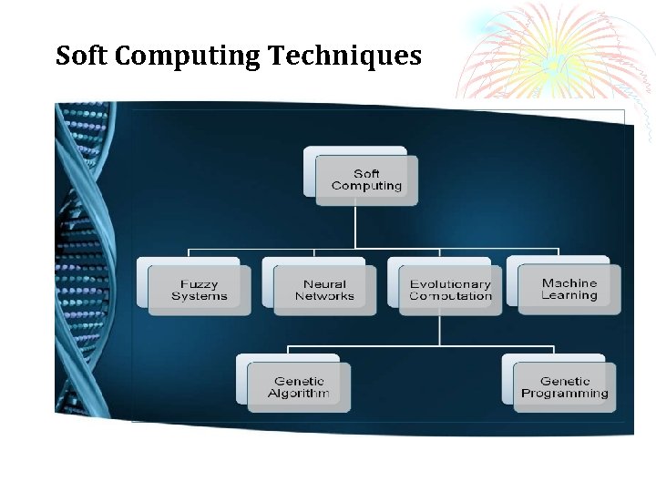
Soft Computing Techniques

Advantages of Evolutionary Computation Ø Ø Ø Conceptual simplicity Broad applicability Hybridization with other methods Parallelism Robust to dynamic changes

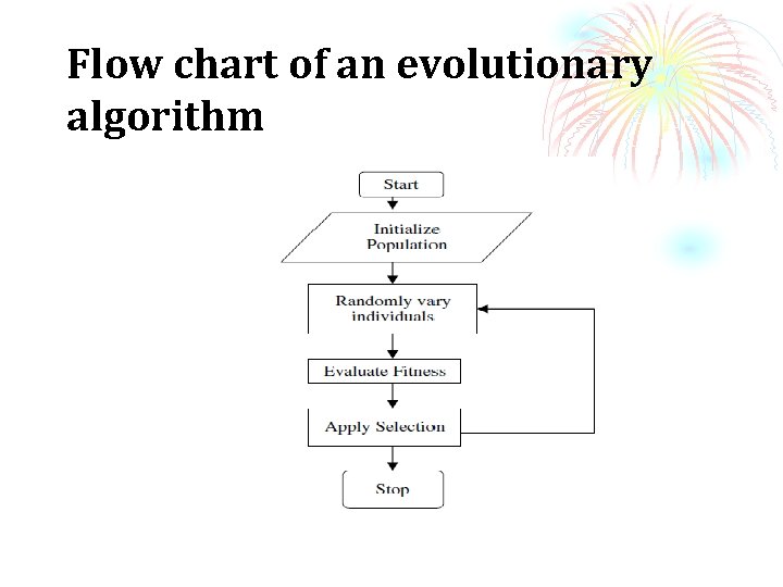
Flow chart of an evolutionary algorithm

Genetic Algorithms - History Ø Pioneered by John Holland in the 1970’s. Ø Got popular in the late 1980’s. Ø Based on ideas from Darwinian Evolution. Ø Can be used to solve a variety of problems that are not easy to solve using other techniques.

Genetic Algorithms Ø An algorithm is a set of instructions that is repeated to solve a problem. Ø A genetic algorithm conceptually follows steps inspired by the biological processes of evolution. Ø Genetic Algorithms follow the idea of SURVIVAL OF THE FITTEST- Better and better solutions evolve from previous generations until a near optimal solution is obtained.

Genetic Algorithm Ø Also known as evolutionary algorithms, genetic algorithms demonstrate self organization and adaptation similar to the way that the fittest biological organism survive and reproduce. Ø A genetic algorithm is an iterative procedure that represents its candidate solutions as strings of genes called chromosomes. Ø Generally applied to spaces which are too large

Genetic Algorithm Ø A genetic algorithm is a search technique used in computing to find true or approximate solution to optimization and search problem. Ø GAs are categorized as global search heuristics. Ø GAs are a particular class of evolutionary algorithms that use techniques inspired by evolutionary biology such as inheritance selection crossover (recombination) and mutation.

Genetic Algorithm Ø The new population is used in the next iteration of the algorithm. Ø The algorithm terminates when either a maximum number of generations has been produced , or a satisfactory fitness level has been reached for the population. Ø The evolution usually starts from a population of randomly generated individuals and happens in generations.

Genetic Algorithm Ø In each generation , the fitness of every individual in the population is evaluated , multiple individuals are selected from the current population (based on their fitness) , and modified to form a new population.

Evolution in the real world Ø Each cell of a living thing contains chromosomes strings of DNA (Dioxy Ribo Nucleic Acid) Ø Each chromosome contains a set of genes - blocks of DNA Ø Each gene determines some aspect of the organism (like eye colour) Ø A collection of genes is sometimes called a genotype Ø A collection of aspects (like eye colour) is sometimes called a phenotype Ø Reproduction involves recombination of genes from parents and then small amounts of mutation (errors) in copying Ø The fitness of an organism is how much it can reproduce before it dies Ø Evolution based on “survival of the fittest”

Concepts Ø Individual: An individual is a single solution. Ø Population: Group of all individuals Ø Chromosome: Genes joined together to form a string of values called chromosome. Ø Gene: A solution to problem represented as a set of parameters , these parameters known as genes. Ø Fitness score (value): Every chromosome has fitness score can be inferred from the chromosome itself by using fitness function. Ø Trait (Allele): Possible aspect (features) of an individual. Ø Genome: Collection of all chromosomes (traits) for an individual. Ø Genotype: The raw genetic information in the chromosome. Ø Phenotype: The expressive of the chromosome in terms of the model.

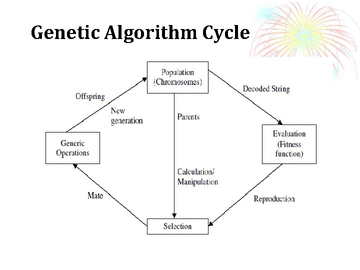
Genetic Algorithm Cycle

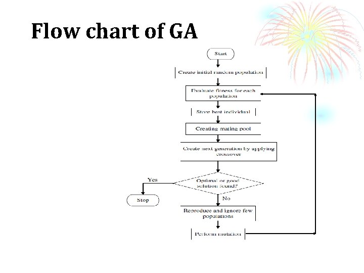
Flow chart of GA

Advantages of GA 1. Parallelism 2. Reliability 3. Solution space is wider 4. The fitness landscape is complex 5. Easy to discover global optimum 6. The problem has multi objective function 7. Only uses function evaluations. 8. Easily modified for different problems. 9. Handles noisy functions well. 10. Handles large, poorly understood search spaces easily

Advantages of GA 11. Good for multi-modal problems Returns a suite of solutions. 12. Very robust to difficulties in the evaluation of the objective function. 13. They require no knowledge or gradient information about the response surface 14. Discontinuities present on the response surface have little effect on overall optimization performance 15. They are resistant to becoming trapped in local optima 16. They perform very well for large-scale optimization problems 17. Can be employed for a wide variety of optimization problems

Limitations of GA 1. The problem of identifying fitness function 2. Definition of representation for the problem 3. Premature convergence occurs 4. The problem of choosing the various parameters like the size of the population, mutation rate, cross over rate, the selection method and its strength. 5. Cannot use gradients. 6. Cannot easily incorporate problem specific information 7. Not good at identifying local optima 8. No effective terminator. 9. Not effective for smooth unimodal functions 10. Needs to be coupled with a local search technique. 11. Have trouble finding the exact global optimum 12. Require large number of response (fitness) function evaluations 13. Configuration is not straightforward

premature convergence means that a population for an optimization problem converged too early, resulting in being suboptimal. In this context, the parental solutions, through the aid of genetic operators, are not able to generate offsprings that are superior to their parents. Premature convergence can happen in case of loss of genetic variation (every individual in the population is identical)

Strategies for preventing premature convergence Ø A mating strategy called incest prevention. Ø Uniform crossover, Ø Favored replacement of similar individuals (preselection or crowding), Ø Segmentation of individuals of similar fitness (fitness sharing), Ø Increasing population size. Ø The genetic variation can also be regained by mutation though this process is highly random.

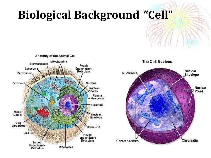
Biological Background “Cell” Ø Every animal cell is a complex of many small “factories” working together. Ø The nucleus in the centre of the cell. Ø The nucleus contains the genetic information.

Biological Background “Cell”

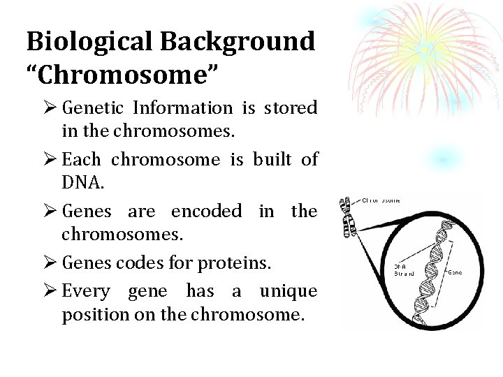
Biological Background “Chromosome” Ø Genetic Information is stored in the chromosomes. Ø Each chromosome is built of DNA. Ø Genes are encoded in the chromosomes. Ø Genes codes for proteins. Ø Every gene has a unique position on the chromosome.

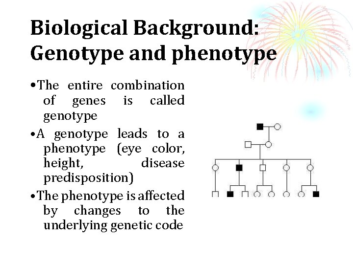
Biological Background: Genotype and phenotype • The entire combination of genes is called genotype • A genotype leads to a phenotype (eye color, height, disease predisposition) • The phenotype is affected by changes to the underlying genetic code

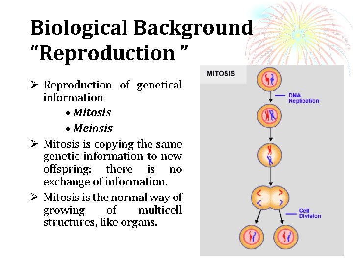
Biological Background “Reproduction ” Ø Reproduction of genetical information • Mitosis • Meiosis Ø Mitosis is copying the same genetic information to new offspring: there is no exchange of information. Ø Mitosis is the normal way of growing of multicell structures, like organs.

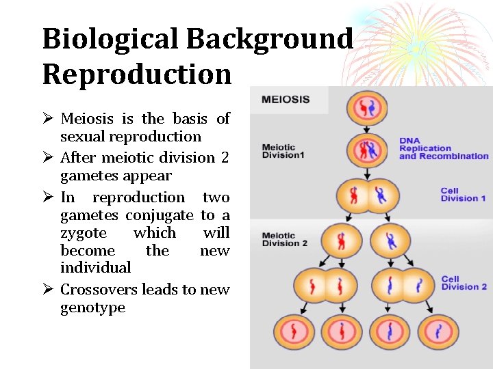
Biological Background Reproduction Ø Meiosis is the basis of sexual reproduction Ø After meiotic division 2 gametes appear Ø In reproduction two gametes conjugate to a zygote which will become the new individual Ø Crossovers leads to new genotype

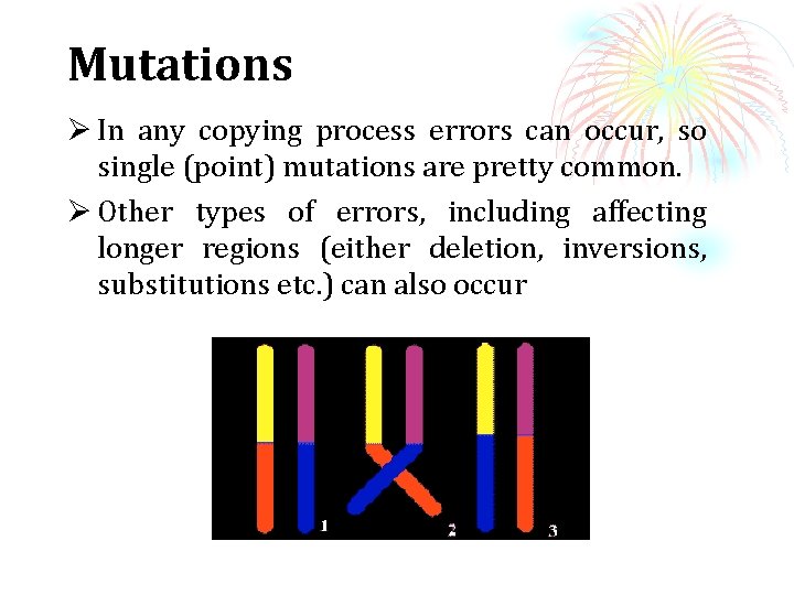
Mutations Ø In any copying process errors can occur, so single (point) mutations are pretty common. Ø Other types of errors, including affecting longer regions (either deletion, inversions, substitutions etc. ) can also occur

“Natural selection” Ø The origin of species: “Preservation of favourable variations and rejection of unfavourable variations. ” Ø There are more individuals born than can survive, so there is a continuous struggle for life. Ø Individuals with an advantage have a greater chance for survive: so survival of the fittest.

GA Steps over an Iteration process SELECTION: The first step consists in selecting individuals for reproduction. This selection is done randomly with a probability depending on the relative fitness of the individuals so that best ones are often chosen for reproduction than poor ones. REPRODUCTION: In the second step, offspring are bred by the selected individuals. For generating new chromosomes, the algorithm can use both recombination and mutation. EVALUATION: Then the fitness of the new chromosomes is evaluated. REPLACEMENT: During the last step, individuals from the old population are killed and replaced by the new ones.

Basic genetic algorithm Ø [start] Genetic random population of n chromosomes (suitable solutions for the problem) Ø [Fitness] Evaluate the fitness f(x) of each chromosome x in the population Ø [New population] Create a new population by repeating following steps until the New population is complete Ø Selection Ø Crossover Ø Mutation Ø Accepting Ø Replace Ø Test [ End condition] Ø Loop [Fitness]

Encoding is a process of representing individual genes. The process can be performed using bits, numbers, trees, arrays, lists or any other objects. The encoding depends mainly on solving the problem. Types of Encoding ØBinary Encoding ØOctal Encoding ØHexadecimal Encoding ØPermutation Encoding (Real Number Coding) ØValue Encoding ØTree Encoding

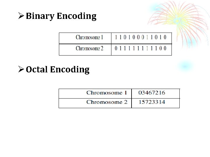
Ø Binary Encoding Ø Octal Encoding

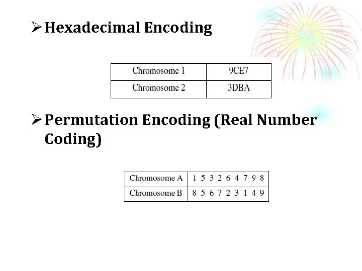
Ø Hexadecimal Encoding Ø Permutation Encoding (Real Number Coding)

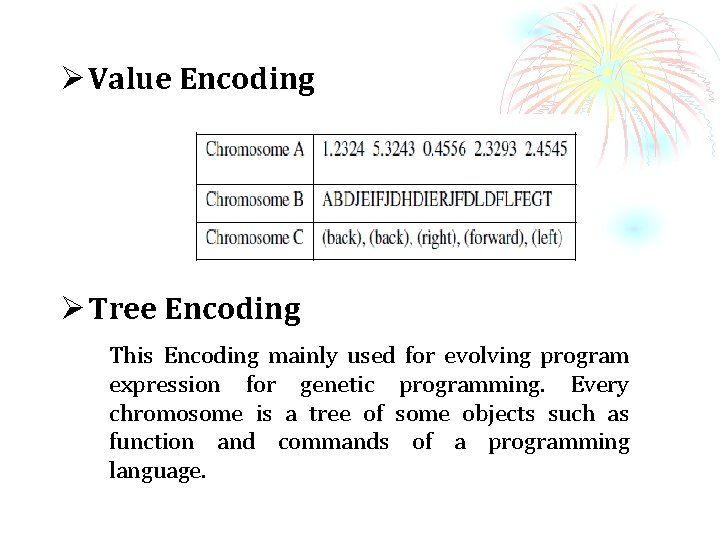
Ø Value Encoding Ø Tree Encoding This Encoding mainly used for evolving program expression for genetic programming. Every chromosome is a tree of some objects such as function and commands of a programming language.

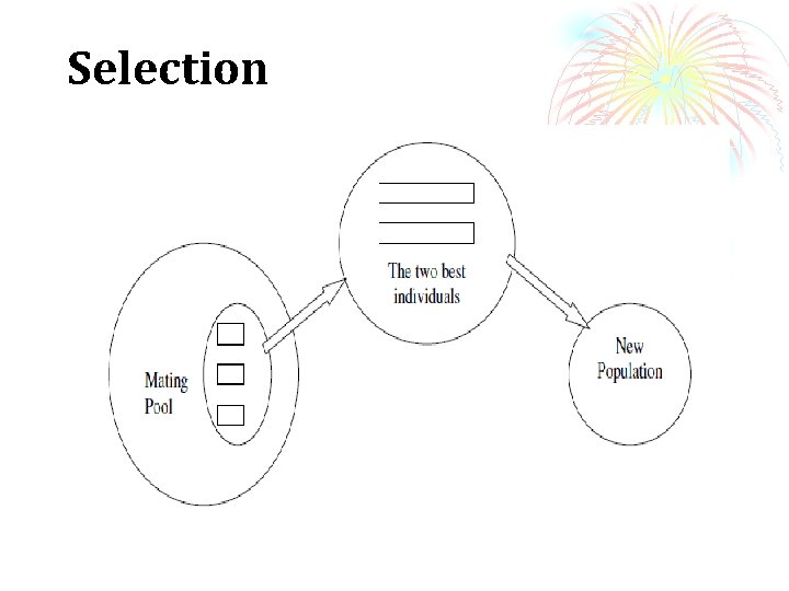
Breeding The breeding process is the heart of the genetic algorithm. It is in this process, the search process creates new and hopefully fitter individuals. The breeding cycle consists of three steps: a. Selecting parents. b. Crossing the parents to create new individuals (offspring or children). c. Replacing old individuals in the population with the new ones.

Selection

Selection Ø Selection is a method that randomly picks chromosomes out of the population according to their evaluation function. Ø The higher the fitness function, the more chance an individual has to be selected. Ø The selection pressure (Selection Intensity) is defined as the degree to which the better individuals are favored. Ø The higher the selection pressured, the more the better individuals are favored. Ø This selection pressure drives the GA to improve the population fitness over the successive generations. Ø Higher selection pressures resulting in higher convergence rates

Selection Ø if the selection pressure is too low, the convergence rate will be slow, and the GA will take unnecessarily longer time to find the optimal solution (Slow finishing). Ø If the selection pressure is too high, there is an increased change of the GA prematurely converging to an incorrect (sub-optimal) solution.

Selection methods Ø Tournament Selection Ø Truncation Selection Ø Linear Ranking Selection Ø Exponential Ranking Selection Ø Elitist Selection Ø Proportional Selection

Selection Schemes Ø Average Fitness Ø Fitness Variance Ø Reproduction Rate Ø Loss of Diversity Ø Selection Intensity Ø Selection Variance

Tournament Selection Tournament selection works as follows Choose some number “t” of individuals randomly from the population and copy the best individual from this group into the intermediate population and repeat N times Often tournaments are held only between two individuals binary tournament but a generalization is possible to an arbitrary group size “t” called tournament size

Truncation Selection In Truncation selection with threshold T only the fraction T best individuals can be selected and they all have the same selection probability This selection method is often used by breeders and in population genetic

Linear Ranking Selection Ranking selection was first suggested by Baker to eliminate the serious disadvantages of proportionate selection. For ranking selection the individuals are sorted according their fitness values and the rank N is assigned to the best individual and the rank to the worst individual. The selection probability is linearly assigned to the individuals according to their rank.

Exponential Ranking Selection Ø Exponential ranking selection differs from linear ranking selection in that the probabilities of the ranked individuals are exponentially weighted Ø The base of the exponent is the parameter 0< c < 1 of the method Ø The closer c is to 1 the lower is the exponentially of the selection method

Elitist Selection Ø The first best chromosome or the few best chromosomes are copied to the new population. Ø The rest is done in a classical way. Such individuals can be lost if they are not selected to reproduce or if crossover or mutation destroys them.

Proportional Selection • The probability of an individual to be selected is simply proportionate to its fitness value

Crossover (Recombination) Ø Crossover is the process of taking two parent solutions and producing from them a child. Ø After the selection (reproduction) process, the population is enriched with better individuals. Ø Reproduction makes clones of good strings but does not create new ones. Ø Crossover operator is applied to the mating pool with the hope that it creates a better offspring.

Crossover (Recombination) Crossover is a recombination operator that proceeds in three steps: i. The reproduction operator selects at random a pair of two individual strings for the mating. ii. A cross site is selected at random along the string length. iii. Finally, the position values are swapped between the two strings following the cross site.

Breeding That is, the simplest way how to do that is to choose randomly some crossover point and copy everything before this point from the first parent and then copy everything after the crossover point from the other parent.

Crossover techniques Ø Single Point Crossover Ø Two Point Crossover Ø Multi-Point Crossover (N-Point crossover) Ø Uniform Crossover Ø Three Parent Crossover Ø Crossover with Reduced Surrogate Ø Shuffle Crossover Ø Precedence Preservative Crossover (PPX) Ø Ordered Crossover Ø Partially Matched Crossover (PMX)

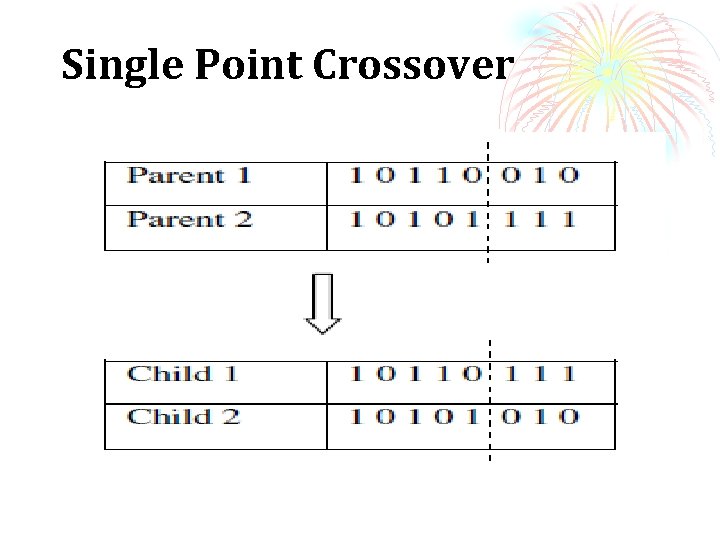
Single Point Crossover

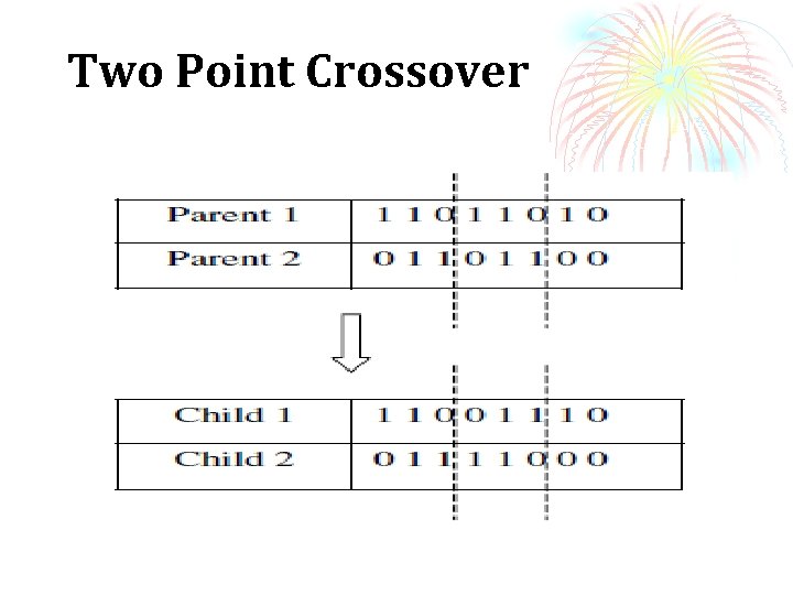
Two Point Crossover

Multi-Point Crossover (NPoint crossover) There are two ways in this crossover. One is even number of cross-sites and the other odd number of cross-sites. In the case of even number of cross-sites, crosssites are selected randomly around a circle and information is exchanged. In the case of odd number of cross-sites, a different cross-point is always assumed at the string beginning.

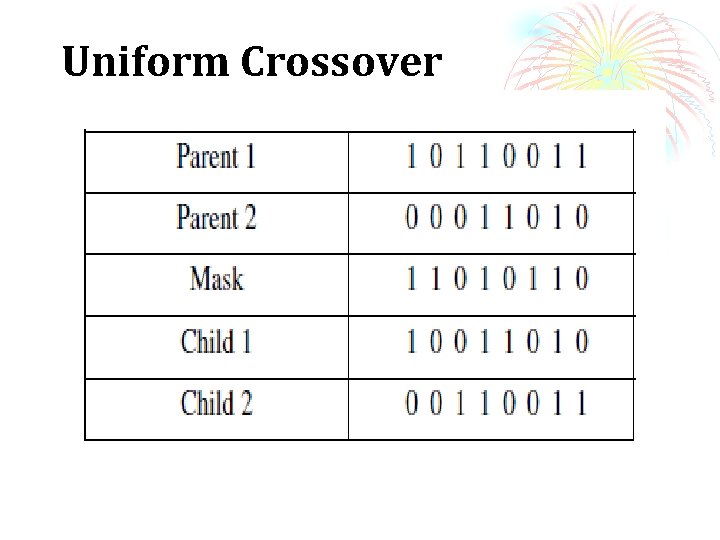
Uniform Crossover

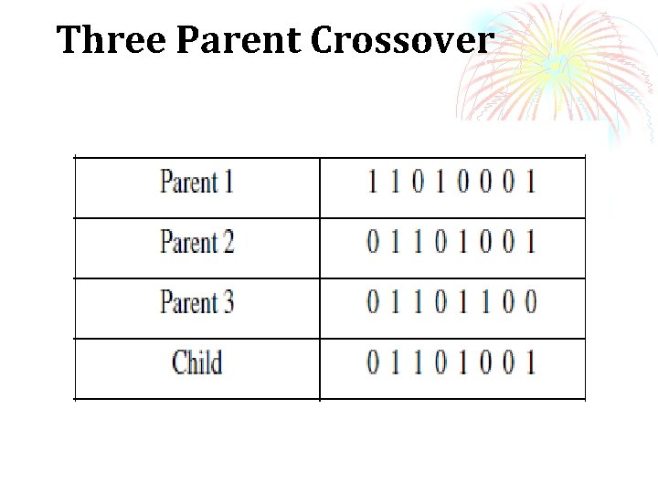
Three Parent Crossover

Crossover with Reduced Surrogate The reduced surrogate operator constrains crossover to always produce new individuals wherever possible. This is implemented by restricting the location of crossover points such that crossover points only occur where gene values differ.

Shuffle Crossover Shuffle crossover is related to uniform crossover. A single crossover position (as in single-point crossover) is selected. But before the variables are exchanged, they are randomly shuffled in both parents. After recombination, the variables in the offspring are un shuffled. This removes positional bias as the variables are randomly reassigned each time crossover is performed.

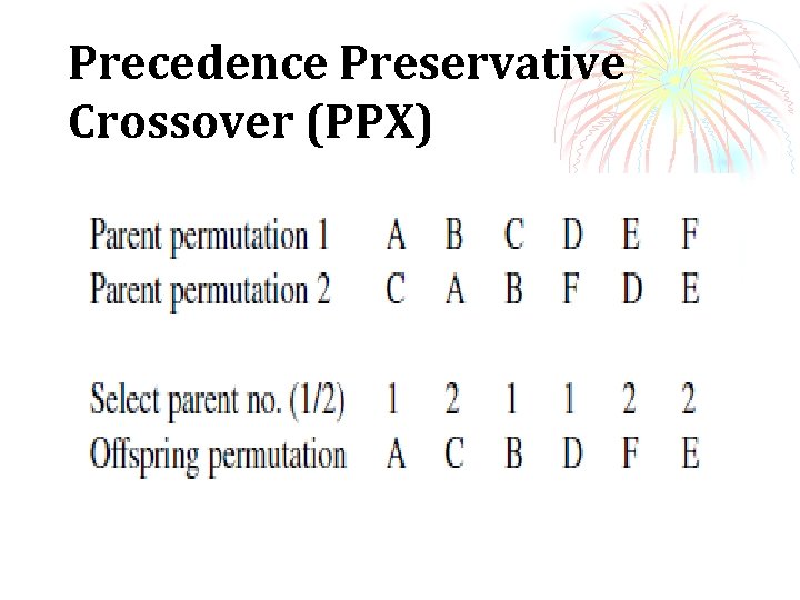
Precedence Preservative Crossover (PPX)

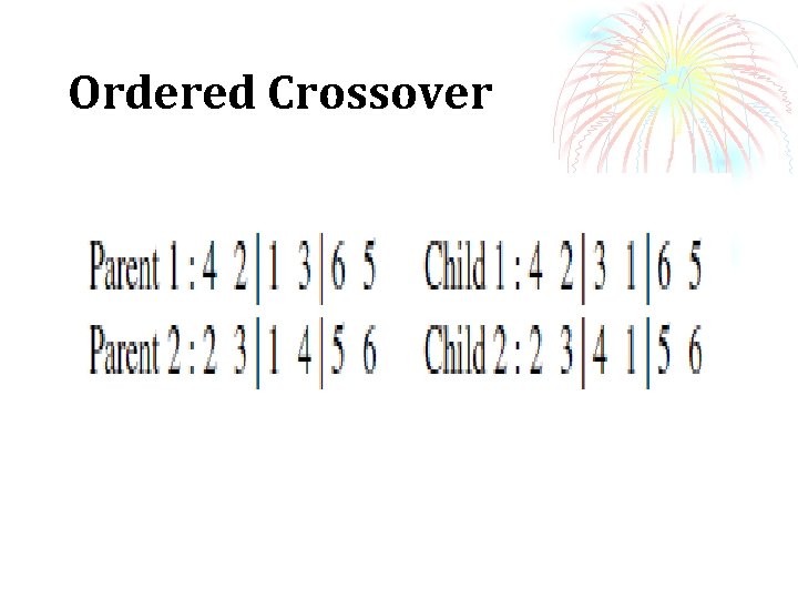
Ordered Crossover

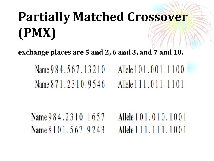
Partially Matched Crossover (PMX) exchange places are 5 and 2, 6 and 3, and 7 and 10.

Crossover Probability The basic parameter in crossover technique is the crossover probability (Pc). Crossover probability is a parameter to describe how often crossover will be performed. Ø If there is no crossover, offspring are exact copies of parents. If there is crossover, offspring are made from parts of both parent’s chromosome. Ø If crossover probability is 100%, then all offspring are made by crossover. Ø If it is 0%, whole new generation is made from exact copies of chromosomes from old population (but this does not mean that the new generation is the same!).

Mutation Ø After crossover, the strings are subjected to mutation. Mutation prevents the algorithm to be trapped in a local minimum. Ø Mutation plays the role of recovering the lost genetic materials as well as for randomly disturbing genetic information. Ø It is an insurance policy against the irreversible loss of genetic material. Mutation has traditionally considered as a simple search operator. Ø If crossover is supposed to exploit the current solution to find better ones, mutation is supposed to help for the exploration of the whole search space. Ø Mutation of a bit involves flipping a bit, changing 0 to 1 and vice-versa.

Mutation Methods Ø Flipping Ø Interchanging Ø Reversing

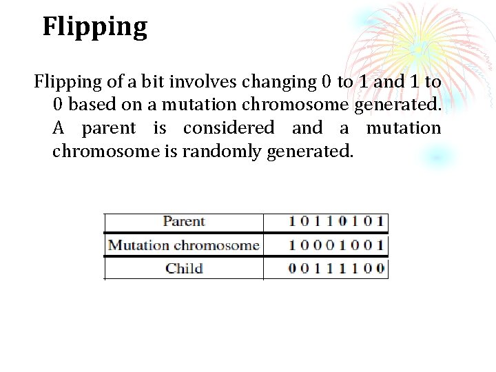
Flipping of a bit involves changing 0 to 1 and 1 to 0 based on a mutation chromosome generated. A parent is considered and a mutation chromosome is randomly generated.

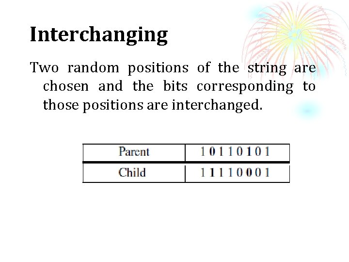
Interchanging Two random positions of the string are chosen and the bits corresponding to those positions are interchanged.

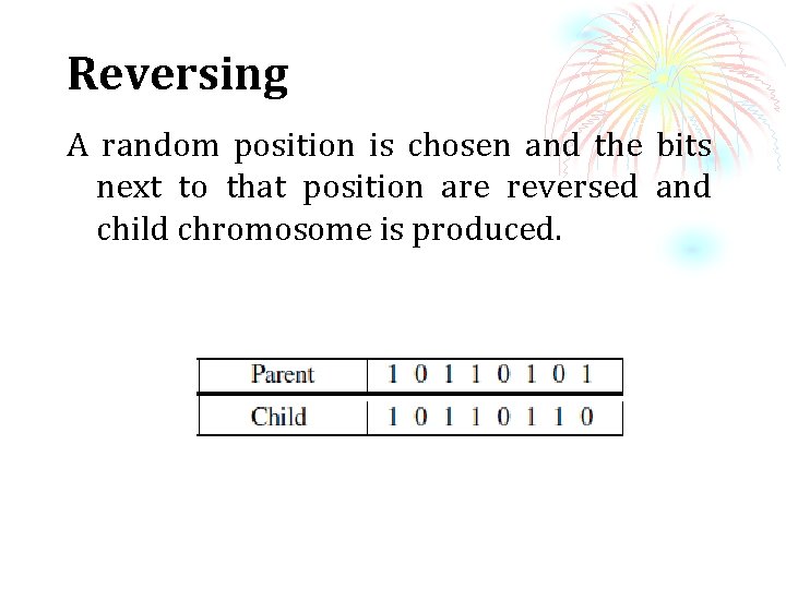
Reversing A random position is chosen and the bits next to that position are reversed and child chromosome is produced.

Mutation Probability Ø The important parameter in the mutation technique is the mutation probability (Pm). Ø The mutation probability decides how often parts of chromosome will be mutated. Ø If there is no mutation, offspring are generated immediately after crossover (or directly copied) without any change. Ø If mutation is performed, one or more parts of a chromosome are changed. If mutation probability is 100%, whole chromosome is changed. Ø if it is 0%, nothing is changed. Ø Mutation generally prevents the GA from falling into local extremes. Ø Mutation should not occur very often, because then GA will in fact change to random search.

Replacement • Replacement is the last stage of any breeding cycle. Two parents are drawn from a fixed size population, they breed two children, but not all four can return to the population, so two must be replaced. The technique used to decide which individual stay in a population and which are replaced in on a par with the selection in influencing convergence. Basically, there are two kinds of methods for maintaining the population; generational updates and steady state updates.

Generational update scheme The basic generational update scheme consists in producing N children from a population of size N to form the population at the next time step (generation), and this new population of children completely replaces the parent selection. Clearly this kind of update implies that an individual can only reproduce with individuals from the same generation.

Steady state update In a steady state update, new individuals are inserted in the population as soon as they are created, as opposed to the generational update where an entire new generation is produced at each time step. The insertion of a new individual usually necessitates the replacement of another population member. The individual to be deleted can be chosen as the worst member of the population.

Random Replacement The children replace two randomly chosen individuals in the population. The parents are also candidates for selection. This can be useful for continuing the search in small populations, since weak individuals can be introduced into the population.

Weak Parent Replacement Ø In weak parent replacement, a weaker parent is replaced by a strong child. Ø With the four individuals only the fittest two, parent or child, return to population.

Both Parents Replacement Both parents replacement is simple. The child replaces the parent. In this case, each individual only gets to breed once. As a result, the population and genetic material moves around but leads to a problem when combined with a selection technique that strongly favors fit parents: the fit breed and then are disposed of.

Search Termination (Convergence Criteria) Ø Maximum generations–The genetic algorithm stops when the specified number of generation’s have evolved. Ø Elapsed time–The genetic process will end when a specified time has elapsed. Note: If the maximum number of generation has been reached before the specified time has elapsed, the process will end. Ø No change in fitness–The genetic process will end if there is no change to the population’s best fitness for a specified number of generations.

Search Termination (Convergence Criteria) Ø Stall generations–The algorithm stops if there is no improvement in the objective function for a sequence of consecutive generations of length Stall generations. Ø Stall time limit–The algorithm stops if there is no improvement in the objective function during an interval of time in seconds equal to Stall time limit.

Methods of termination techniques. Ø Best Individual: A best individual convergence criterion stops the search once the minimum fitness in the population drops below the convergence value. This brings the search to a faster conclusion guaranteeing at least one good solution. Ø Worst individual: Worst individual terminates the search when the least fit individuals in the population have fitness less than the convergence criteria. This guarantees the entire population to be of minimum standard, although the best individual may not be significantly better than the worst. In this case, a stringent convergence value may never be met, in which case the search will terminate after the maximum has been exceeded.

Methods of termination techniques. Ø Sum of Fitness: In this termination scheme, the search is considered to have satisfaction converged when the sum of the fitness in the entire population is less than or equal to the convergence value in the population record. Ø Median Fitness: Here at least half of the individuals will be better than or equal to the convergence value, which should give a good range of solutions to choose from.

Why do Genetic Algorithms Work? The search heuristics of GA are based upon Holland’s scheme theorem. A schema is defined as templates for describing a subset of chromosomes with similar sections. The schemata consist of bits 0, 1 and metacharacter. The template is a suitable way of describing similarities among Patterns in the chromosomes Holland derived an expression that predicts the number of copies of a particular schema would have in the next generation after undergoing exploitation, crossover and mutation.

Why do Genetic Algorithms Work? It should be noted that particularly good schemata will propagate in future generations. Thus, schema that are low-order, well defined and have above average fitness are preferred and are termed building blocks. This leads to a building block principle of GA: low order, welldefined, average fitness schemata will combine through crossover to form high order, above average fitness schemata. Since GAs process may schemata in a given generation they are said to have the property of implicit parallelism.

Building Block Hypothesis Schemata with high fitness values and small defining are called Building Blocks. The most obvious interpretation is that a schema is highly fit if its average fitness considerably higher than the average fitness of all strings in the search space. This version of the building block hypothesis might be called the “static building block hypothesis”. Another interpretation is that a schema is highly fit if the average fitness of the schema representatives in the populations of the GA run is higher than the average fitness of all individuals in these populations. This might be called the “relative building block hypothesis”.

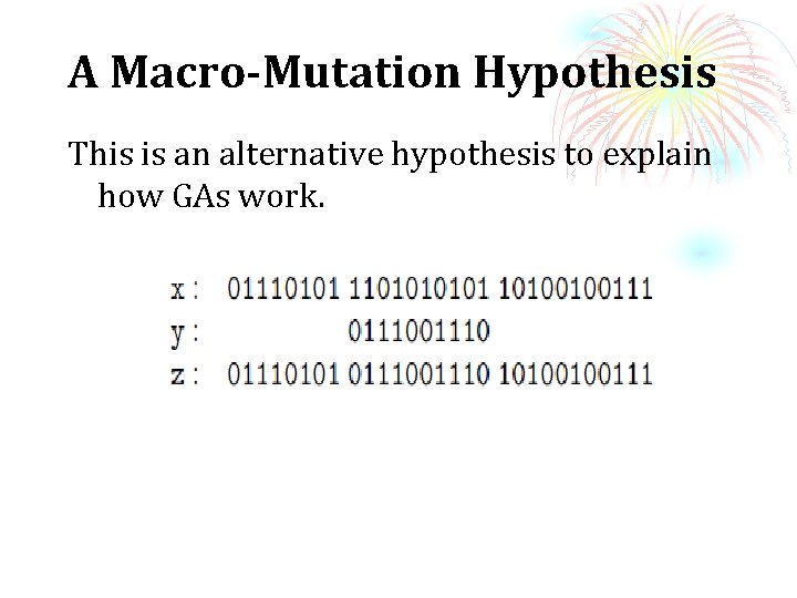
A Macro-Mutation Hypothesis This is an alternative hypothesis to explain how GAs work.

An Adaptive Mutation Hypothesis An adaptive mutation hypothesis is that where crossover in a GA serves as a mutation mechanism that is automatically adapted to the stage of convergence of the population. Crossover produces new individuals in the same region as the current population. Thus, as the population “converges” into a smaller region of the search space, crossover produces new individuals within this region. Thus, crossover can be considered as an adaptive mutation method that reduces the strength of mutation as the run progresses.

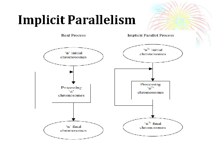
The Schema Theorem A schema is a similarity template describing a subset of string displaying similarities at certain string positions. In general, there are 21 different strings or chromosome of length 1, but schemata display an order of 31. A particular string of length 1 inside a population of ‘n’ individuals into one of the 21 schemata can be obtained from this string. Thus, in the entire population the number of schemata present in each generation is somewhere between 21 and n. 21, depending upon the population diversity. J. Holland estimated that in a population of ‘n’ chromosomes, the Gas process O(n 3) schemata into each generation. This is called as implicit parallel process.

The Schema Theorem A schema represents an affined variety of the search space: for example the schema 01**11*0 is a sub-space of the space of codes of 8 bits length (∗ can be 0 or 1). The GA modeled in schema theory is a canonical GA, which acts on binary strings, and for which the creation of a new generation is based on three operators: Ø A proportionate selection, where the fitness function steps in: the probability that a solution of the current population is selected and is proportional to its fitness. Ø The genetic operators: single point crossover and bitflip mutation, randomly applied with probabilities pc and pm.

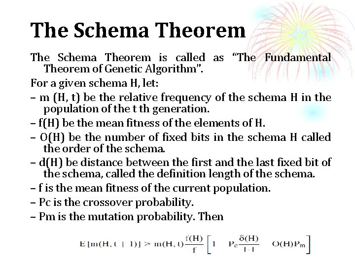
The Schema Theorem is called as “The Fundamental Theorem of Genetic Algorithm”. For a given schema H, let: – m (H, t) be the relative frequency of the schema H in the population of the t th generation. – f(H) be the mean fitness of the elements of H. – O(H) be the number of fixed bits in the schema H called the order of the schema. – d(H) be distance between the first and the last fixed bit of the schema, called the definition length of the schema. – f is the mean fitness of the current population. – Pc is the crossover probability. – Pm is the mutation probability. Then

Application of schema theorem Ø It provides some tools to check whether a given representation is well-suited to a GA. Ø The analysis of nature of the “good” schemata gives few ideas on the efficiency of genetic algorithm.

Implicit Parallelism Even though at each generation one performs a proportional computation to the size of the population n, we obtain useful processing of n 3 schemata’s in parallel with memory other than the population itself. At present, the common interpretation is that a GA processes an enormous amount of schemata implicitly.

Implicit Parallelism

Solution Evaluation At the end of the search genetic algorithm displays the final population with their fitnesses, from which it is possible to select a solution and write it back to the system for further generations. In certain systems it is not always practical to declare all the necessary parameters after the search, or perhaps some factors were simply overlooked. Thus once if a solution is obtained, it has to be evaluated for all its various parameters under consideration, which includes fitnesses, median fitness, best individual, maximum fitness and so on.

Search Refinement Search parameters like selection, crossover and replacement, which are very effective in the early stages of a search, may not necessarily be the best toward the end of the search. During early search it is desirable to get good spread of points through the solution space in order to find at least the beginning of the various optima. Once the population starts converging on optima it might be better to exercise more stringent selection and replacement to completely cover that region of space. Alternatively, refinement can also be made in the domain and resolution of the individual genes.

Constraints In case of constrained optimization problems, the information’s are provided for the variables under consideration. Constraints are classified as, 1. Equality relations. 2. Inequality relations.

Fitness Scaling Fitness scaling is performed in order to avoid premature convergence and slow finishing. The various types of fitness scaling are: 1. Linear scaling 2. σ–Truncation 3. Power law.

Linear Scaling Consider, f – Unscaled raw fitness f ’– Fitness after scaling f ’ = af + b

σ–Truncation “σ–Truncation” discards such off the average members. Linear scaling is then applied to the remaining members. f” = f − (fav-C σ) if RHS > 0 = 0, otherwise. After this linear scaling is applied without the danger of negative fitness. f’ = af” + b

Power law. In power law scaling, the scaled fitness is given by, Scaled fitness f’ = fk(raw fitness f) K–problem dependent constant. 1. 005

Niching Genetic Algorithms Ø Multimodal Optimization Ø Traditional genetic algorithms with elitist selection are suitable to locate the optimum of unimodal functions as they converge to a single solution of the search space. Ø Real problem, however, often require the identification of optima along with some local optima. Ø For this purpose, niching methods extend the simple genetic algorithms by promoting the formation of subpopulations in the neighborhood of the local optimal solutions.

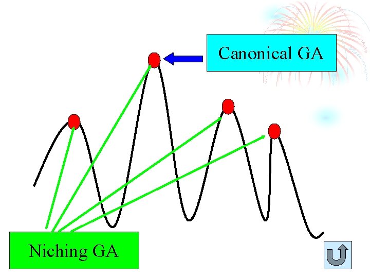
Canonical GA Niching GA

Niching Genetic Algorithms Ø Niching methods have been developed to reduce the effect of genetic drift resulting from the selection operator in the simple genetic algorithms. Ø They maintain population diversity and permit genetic algorithms to explore more search space so as to identify multiple peaks, whether optimal or otherwise. Ø The fitness sharing method is probably the best known and best used among the niching techniques.

Ecological Meaning Ø In natural ecosystem, a niche can be viewed as an organisms task, which permits species to survive in their environment. Ø Species are defined as a collection of similar organisms with similar features. Ø The subdivision of environment on the basis of an organisms role reduces inter-species competition for environmental resources. Ø This reduction in competition helps stable subpopulations to form around different niches in the environment.

Analogy • By analogy, in multimodal GAs, a niche is commonly referred to as the location of each optimum in the search space and the fitness representing the resource of that niche.

Niching Methods Ø The Fitness Sharing Method Ø Crowding Method Ø Clearing Method

The Fitness Sharing Method Ø The sharing method essentially modifies the search landscape by reducing the payoff in densely populated regions. Ø This method rewards individuals that uniquely exploit areas of the domain, while discouraging highly similar individuals in a domain. Ø This causes population diversity pressure, which helps maintain population members at local optima.

The Crowding Method Ø Standard Crowding Method (De. Jong, 1975) Ø Deterministic Crowding Method (Mahfoud, 1995)

Standard Crowding Method Ø Standard crowding method was proposed by De. Jong (1975). Ø In this method, only a fraction of the global population specified by a percentage G (generation gap) reproduces and dies in each generation. Ø An offspring replaces the most similar individual (in terms of genotype comparison) taken from a randomly drawn subpopulation of size CF (crowding factor) from the global population. Ø This method has been found to be limited in multimodal function optimization.

Deterministic Crowing Method Ø Mahfoud (1995) improved De. Jong's standard crowding and propose his deterministic crowding method. Ø Deterministic crowding method introduces competition between children and parents of identical niches. Ø This method tends to identify solutions with higher fitness and lose solutions with lower fitness.

Clearing Method Ø Clearing method was proposed by Petrowski (1996, 1997) based on limited resources of environment. Ø Instead of evenly sharing the available resources among the individuals of a subpopulation, the clearing procedure supplies these resources only to the best individuals of each subpopulation. Ø Clearing method is found to be most suitable to deal with the extremely complicated search space of the portfolio optimization problem.

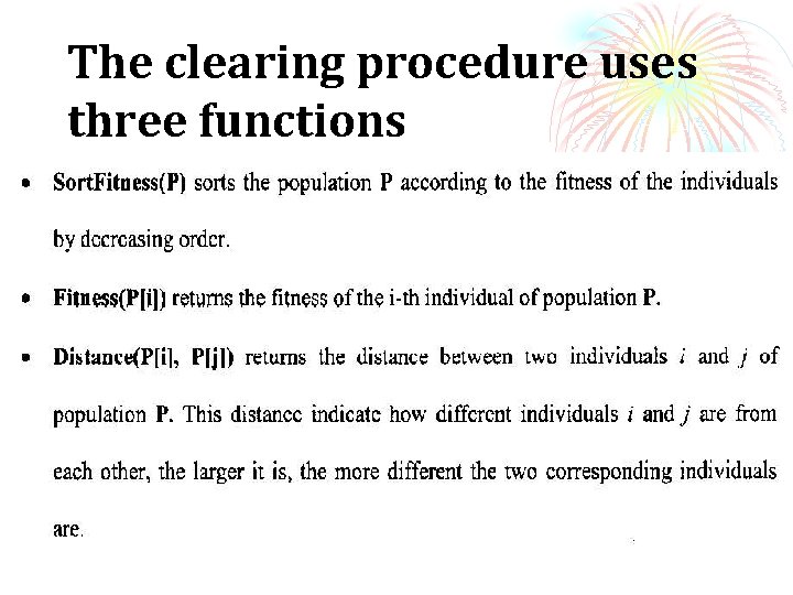
The clearing procedure uses three functions

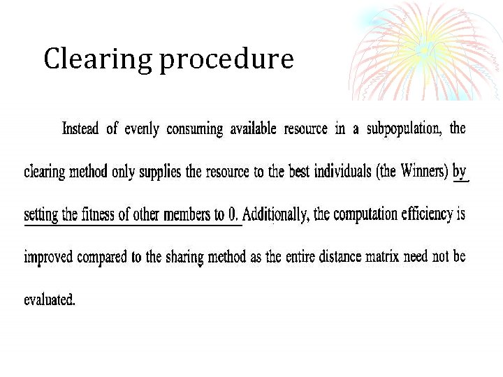
Clearing procedure

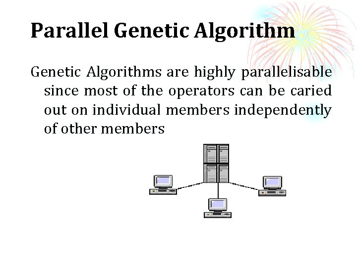
Parallel Genetic Algorithms are highly parallelisable since most of the operators can be caried out on individual members independently of other members

Parallel Genetic Algorithm There are two main possible methods to parallelism. Ø The first of which is data parallelism, where the same instruction will be executed on numerous data simultaneously. Ø The second one is control parallelism which involves execution of various instructions concurrently

Parallel Genetic Algorithm GAs can be parallelized depending on the following: Ø How to evaluate the fitness and how to apply the genetic operators Ø Is it a single population or multiple subpopulations? Ø In case of multiple subpopulations how the individuals will be exchanged Ø How to apply the selection (local/global)

Types of Genetic Algorithm Ø Global Populations with Parallelism Ø Island Models Ø Cellular Genetic Algorithms

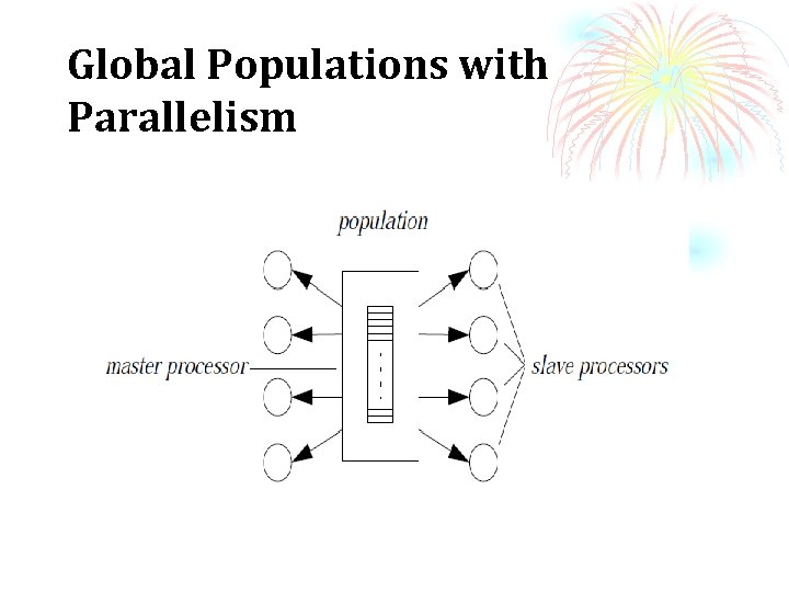
Global Populations with Parallelism In these models one global population is kept, on which the traditional genetic operators are performed. Selection is done on the global population, and then the selected individuals undergo crossover and mutation in parallel. Types of Global Populations with Parallelism Ø synchronous master-slave Ø Semi-synchronous master-slave Ø asynchronous concurrent

Global Populations with Parallelism

Island Models Looking at nature again one could say that the world of humans consists of one big population. Another view is to say that it’s actually a collection of subpopulations which evolve independently from each other on isolated continents or in restricted regions. Once in a while some individuals from one region migrate to another region. This migration allows subpopulations to share genetic material. The idea is that isolated environments, or competing islands, are more search-effective than a wider one in which all the members are held together.

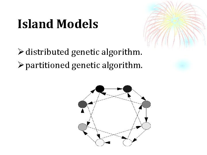
Island Models Ø distributed genetic algorithm. Ø partitioned genetic algorithm.

Cellular Genetic Algorithms Genetic algorithms implemented on a SIMD machine typically have one individual string residing at each processor element (cells). Individuals select mates and recombine with other individuals in their immediate neighbourhood (e. g. north, south, east and west). This class of genetic algorithms are in fact a subclass of cellular automata. Thus, the term Cellular Genetic Algorithm is proposed to describe this class of parallel algorithms.

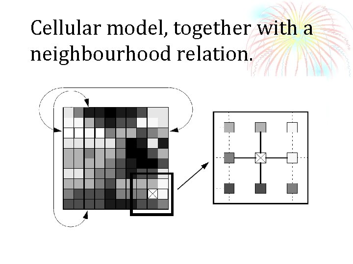
Cellular model, together with a neighbourhood relation.