Bioinformatics Unsupervised Datamining Mark Gerstein Yale University gersteinlab

Bioinformatics: Unsupervised Datamining Mark Gerstein, Yale University gersteinlab. org/courses/452 (last edit in spring ’ 16)

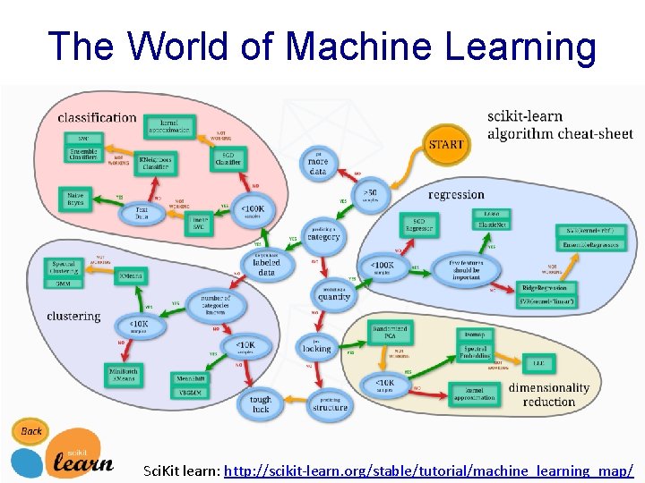
The World of Machine Learning Sci. Kit learn: http: //scikit-learn. org/stable/tutorial/machine_learning_map/

Abstract Overview: Supervised vs Unsupervised Mining

Structure of Genomic Features Matrix

Represent predictors in abstract high dimensional space

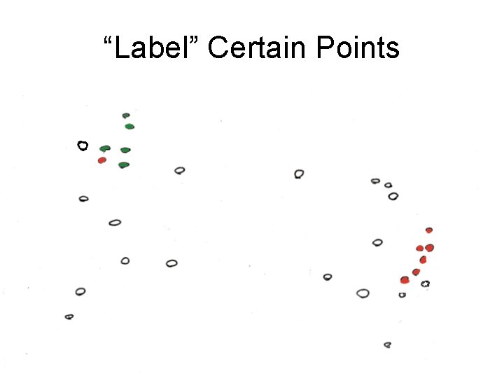
“Label” Certain Points

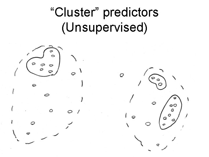
“Cluster” predictors (Unsupervised)

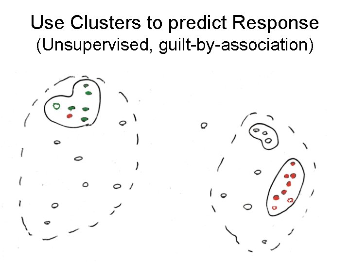
Use Clusters to predict Response (Unsupervised, guilt-by-association)

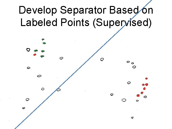
Develop Separator Based on Labeled Points (Supervised)

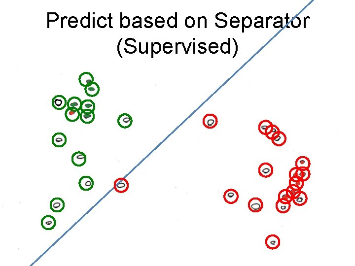
Predict based on Separator (Supervised)

Unsupervised Mining – Simple overlaps & enriched regions – Clustering rows & columns (networks) – PCA – SVD (theory + appl. ) – Weighted Gene Co-Expression Network – Biplot – CCA

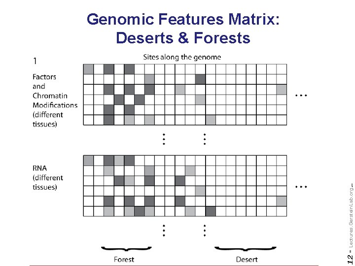
Do not reproduce without permission 12 - Lectures. Gerstein. Lab. org (c) '09 Genomic Features Matrix: Deserts & Forests

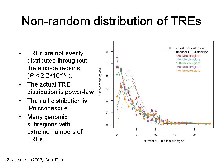
Non-random distribution of TREs • TREs are not evenly distributed throughout the encode regions (P < 2. 2× 10− 16 ). • The actual TRE distribution is power-law. • The null distribution is ‘Poissonesque. ’ • Many genomic subregions with extreme numbers of TREs. Zhang et al. (2007) Gen. Res.

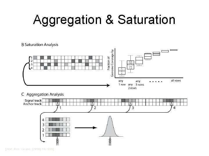
Aggregation & Saturation [Nat. Rev. Genet. (2010) 11: 559]

Unsupervised Mining Clustering Columns & Rows of the Data Matrix

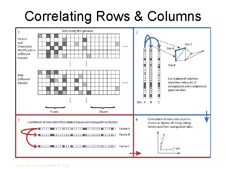
Correlating Rows & Columns [Nat. Rev. Genet. (2010) 11: 559]

Spectral Methods Outline & Papers • • • Simple background on PCA (emphasizing lingo) More abstract run through on SVD Application to – O Alter et al. (2000). "Singular value decomposition for genomewide expression data processing and modeling. " PNAS 97: 10101 – Langfelder P, Horvath S (2007) Eigengene networks for studying the relationships between co-expression modules. BMC Systems Biology 2007, 1: 54 – Z Zhang et al. (2007) "Statistical analysis of the genomic distribution and correlation of regulatory elements in the ENCODE regions. " Genome Res 17: 787 – TA Gianoulis et al. (2009) "Quantifying environmental adaptation of metabolic pathways in metagenomics. " PNAS 106: 1374.

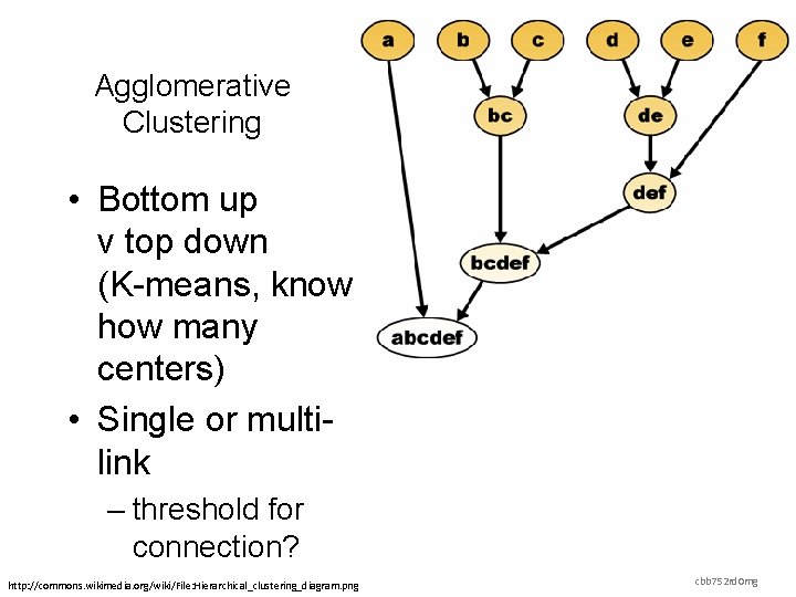
Agglomerative Clustering • Bottom up v top down (K-means, know how many centers) • Single or multilink – threshold for connection? http: //commons. wikimedia. org/wiki/File: Hierarchical_clustering_diagram. png cbb 752 rd 0 mg

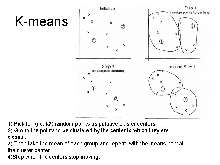
K-means 1) Pick ten (i. e. k? ) random points as putative cluster centers. 2) Group the points to be clustered by the center to which they are closest. 3) Then take the mean of each group and repeat, with the means now at the cluster center. 4)Stop when the centers stop moving.

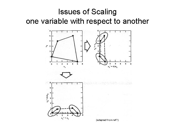
Issues of Scaling one variable with respect to another (adapted from ref? )

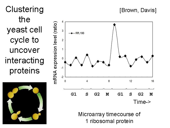
[Brown, Davis] m. RNA expression level (ratio) Clustering the yeast cell cycle to uncover interacting proteins Time-> Microarray timecourse of 1 ribosomal protein

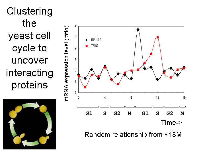
m. RNA expression level (ratio) Clustering the yeast cell cycle to uncover interacting proteins Time-> Random relationship from ~18 M

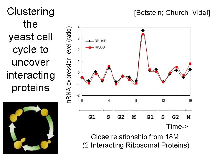
[Botstein; Church, Vidal] m. RNA expression level (ratio) Clustering the yeast cell cycle to uncover interacting proteins Time-> Close relationship from 18 M (2 Interacting Ribosomal Proteins)

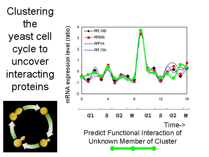
m. RNA expression level (ratio) Clustering the yeast cell cycle to uncover interacting proteins Time-> Predict Functional Interaction of Unknown Member of Cluster

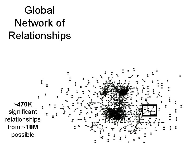
Global Network of Relationships ~470 K significant relationships from ~18 M possible

Network = Adjacency Matrix • Adjacency matrix A=[aij] encodes whether/how a pair of nodes is connected. • For unweighted networks: entries are 1 (connected) or 0 (disconnected) • For weighted networks: adjacency matrix reports connection strength between gene pairs Adapted from : http: //www. genetics. ucla. edu/labs/horvath/Coexpression. Network

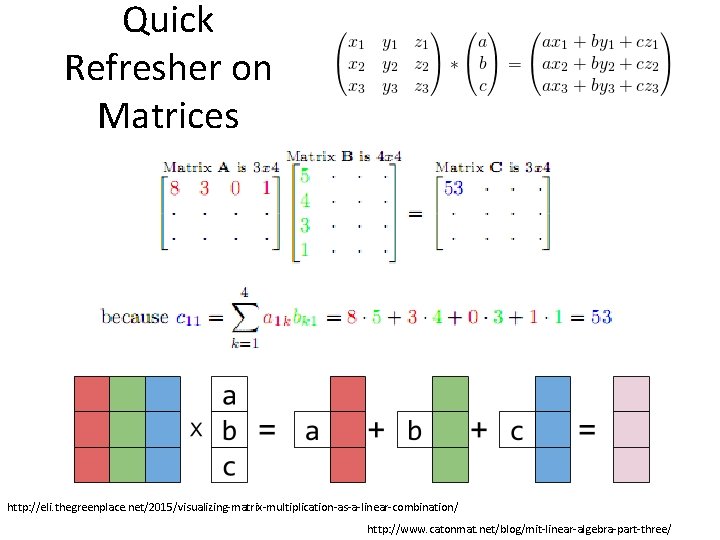
Quick Refresher on PCA/Matrices

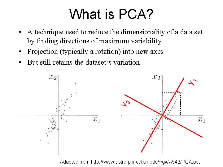
What is PCA? y 2 y 1 • A technique used to reduce the dimensionality of a data set by finding directions of maximum variability • Projection (typically a rotation) into new axes • But still retains the dataset’s variation Adapted from http: //www. astro. princeton. edu/~gk/A 542/PCA. ppt

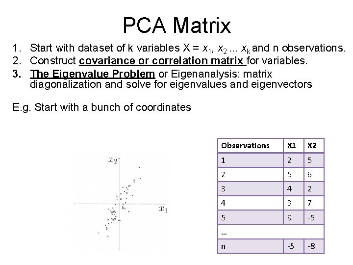
PCA Matrix 1. Start with dataset of k variables X = x 1, x 2. . . xk and n observations. 2. Construct covariance or correlation matrix for variables. 3. The Eigenvalue Problem or Eigenanalysis: matrix diagonalization and solve for eigenvalues and eigenvectors E. g. Start with a bunch of coordinates Observations X 1 X 2 1 2 5 6 3 4 2 4 3 7 5 9 -5 -5 -8 … n

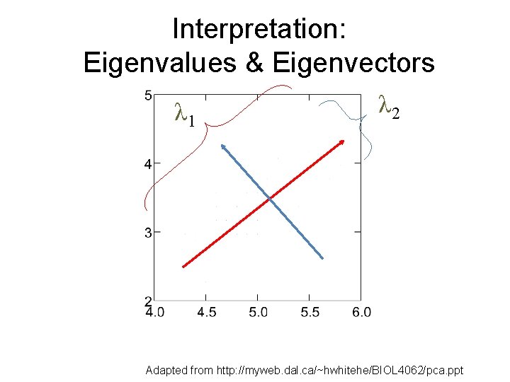
Interpretation: Eigenvalues & Eigenvectors λ 1 λ 2 Adapted from http: //myweb. dal. ca/~hwhitehe/BIOL 4062/pca. ppt

Quick Refresher on Matrices http: //eli. thegreenplace. net/2015/visualizing-matrix-multiplication-as-a-linear-combination/ http: //www. catonmat. net/blog/mit-linear-algebra-part-three/

Unsupervised Mining SVD Puts together slides prepared by Brandon Xia with images from Alter et al. papers

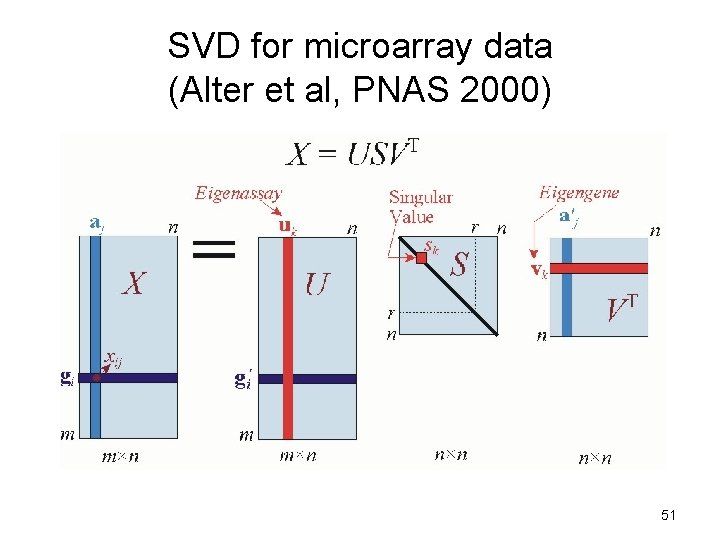
SVD for microarray data (Alter et al, PNAS 2000) 33

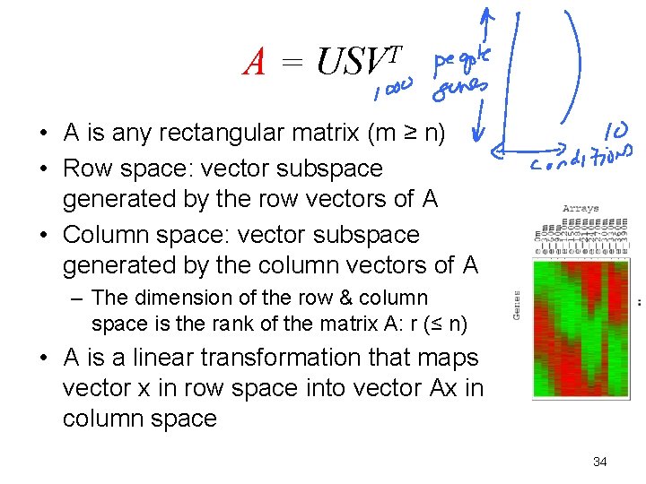
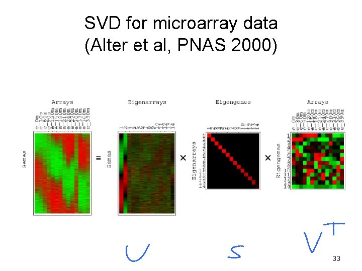
A = USVT • A is any rectangular matrix (m ≥ n) • Row space: vector subspace generated by the row vectors of A • Column space: vector subspace generated by the column vectors of A – The dimension of the row & column space is the rank of the matrix A: r (≤ n) • A is a linear transformation that maps vector x in row space into vector Ax in column space 34

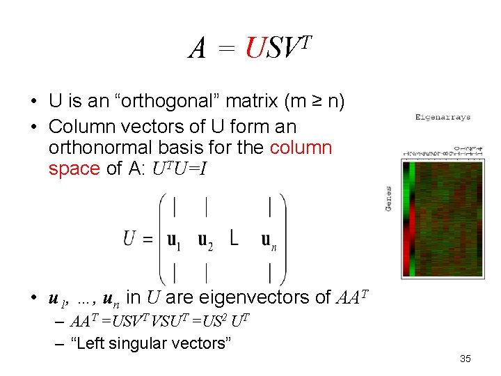
A = USVT • U is an “orthogonal” matrix (m ≥ n) • Column vectors of U form an orthonormal basis for the column space of A: UTU=I • u 1, …, un in U are eigenvectors of AAT – AAT =USVT VSUT =US 2 UT – “Left singular vectors” 35

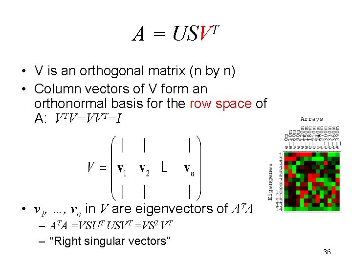
A = USVT • V is an orthogonal matrix (n by n) • Column vectors of V form an orthonormal basis for the row space of A: VTV=VVT=I • v 1, …, vn in V are eigenvectors of ATA – ATA =VSUT USVT =VS 2 VT – “Right singular vectors” 36

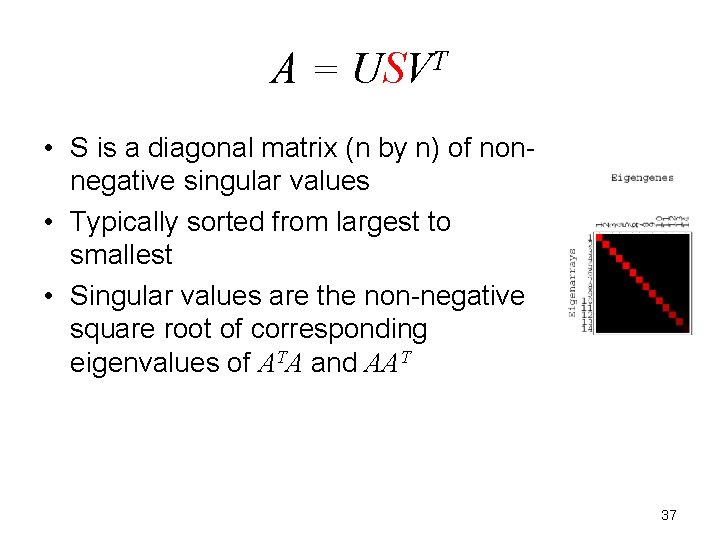
A = USVT • S is a diagonal matrix (n by n) of nonnegative singular values • Typically sorted from largest to smallest • Singular values are the non-negative square root of corresponding eigenvalues of ATA and AAT 37

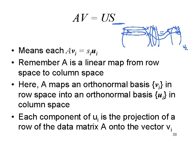
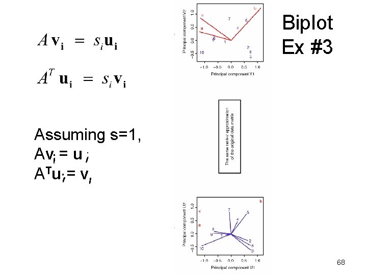
AV = US • Means each Avi = siui • Remember A is a linear map from row space to column space • Here, A maps an orthonormal basis {vi} in row space into an orthonormal basis {ui} in column space • Each component of ui is the projection of a row of the data matrix A onto the vector vi 38

SVD of A (m by n): recap • A = USVT = (big-"orthogonal")(diagonal)(sq-orthogonal) • u 1, …, um in U are eigenvectors of AAT • v 1, …, vn in V are eigenvectors of ATA • s 1, …, sn in S are nonnegative singular values of A • AV = US means each Avi = siui • “Every A is diagonalized by 2 orthogonal matrices” 39

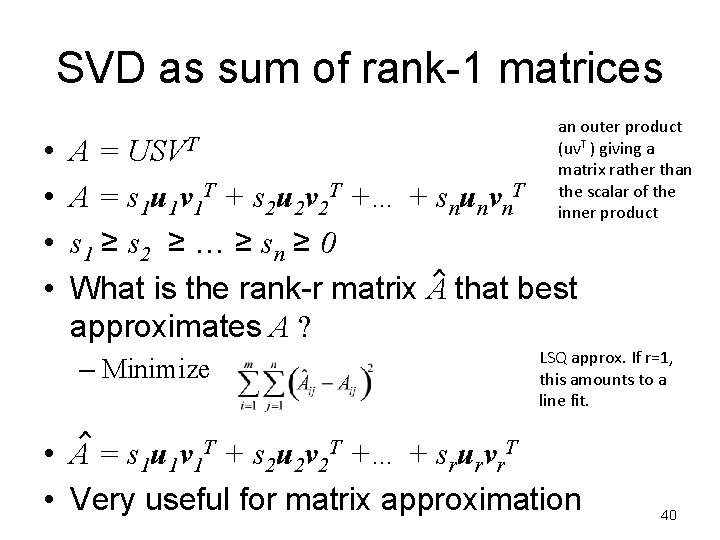
SVD as sum of rank-1 matrices • • an outer product (uv. T ) giving a matrix rather than the scalar of the inner product A = USVT A = s 1 u 1 v 1 T + s 2 u 2 v 2 T +… + snunvn. T s 1 ≥ s 2 ≥ … ≥ sn ≥ 0 What is the rank-r matrix A that best approximates A ? – Minimize LSQ approx. If r=1, this amounts to a line fit. • A = s 1 u 1 v 1 T + s 2 u 2 v 2 T +… + srurvr. T • Very useful for matrix approximation 40

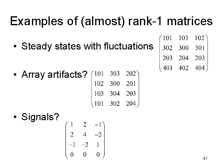
Examples of (almost) rank-1 matrices • Steady states with fluctuations • Array artifacts? • Signals? 41

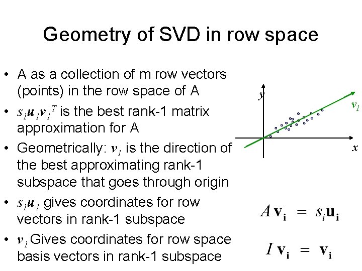
Geometry of SVD in row space • A as a collection of m row vectors (points) in the row space of A • s 1 u 1 v 1 T is the best rank-1 matrix approximation for A • Geometrically: v 1 is the direction of the best approximating rank-1 subspace that goes through origin • s 1 u 1 gives coordinates for row vectors in rank-1 subspace • v 1 Gives coordinates for row space basis vectors in rank-1 subspace y v 1 x

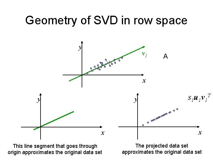
Geometry of SVD in row space y v 1 A x y y x This line segment that goes through origin approximates the original data set s 1 u 1 v 1 T x The projected data set approximates the original data set

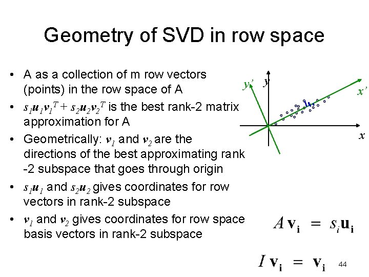
Geometry of SVD in row space • A as a collection of m row vectors y y’ (points) in the row space of A • s 1 u 1 v 1 T + s 2 u 2 v 2 T is the best rank-2 matrix approximation for A • Geometrically: v 1 and v 2 are the directions of the best approximating rank -2 subspace that goes through origin • s 1 u 1 and s 2 u 2 gives coordinates for row vectors in rank-2 subspace • v 1 and v 2 gives coordinates for row space basis vectors in rank-2 subspace x’ x 44

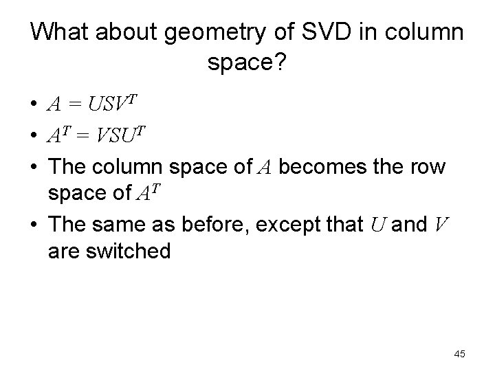
What about geometry of SVD in column space? • A = USVT • AT = VSUT • The column space of A becomes the row space of AT • The same as before, except that U and V are switched 45

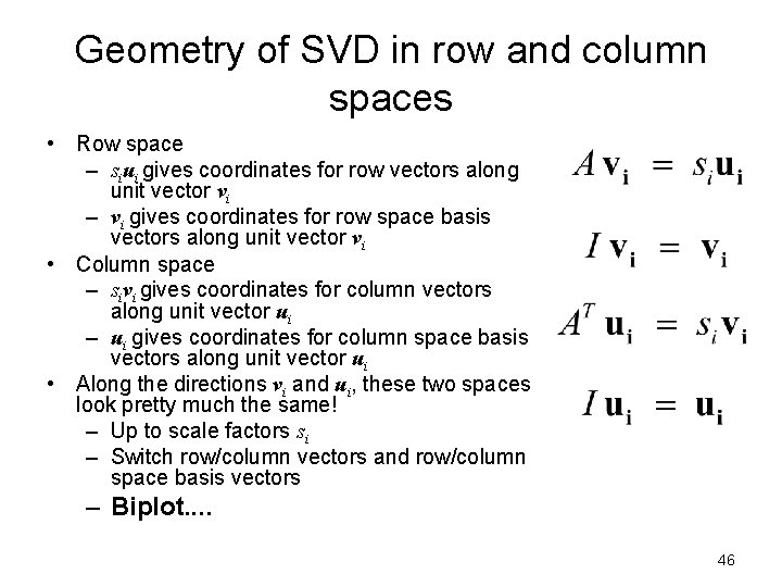
Geometry of SVD in row and column spaces • Row space – siui gives coordinates for row vectors along unit vector vi – vi gives coordinates for row space basis vectors along unit vector vi • Column space – sivi gives coordinates for column vectors along unit vector ui – ui gives coordinates for column space basis vectors along unit vector ui • Along the directions vi and ui, these two spaces look pretty much the same! – Up to scale factors si – Switch row/column vectors and row/column space basis vectors – Biplot. . 46

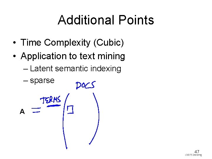
Additional Points • Time Complexity (Cubic) • Application to text mining – Latent semantic indexing – sparse A 47 cbb 752 rd 0 mg

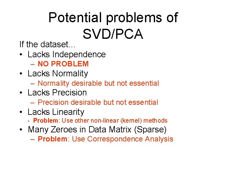
Potential problems of SVD/PCA If the dataset… • Lacks Independence – NO PROBLEM • Lacks Normality – Normality desirable but not essential • Lacks Precision – Precision desirable but not essential • Lacks Linearity - Problem: Use other non-linear (kernel) methods • Many Zeroes in Data Matrix (Sparse) – Problem: Use Correspondence Analysis

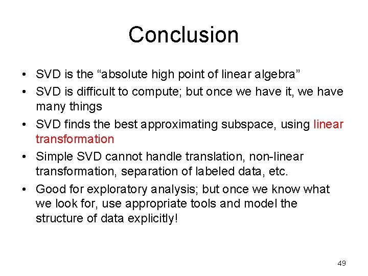
Conclusion • SVD is the “absolute high point of linear algebra” • SVD is difficult to compute; but once we have it, we have many things • SVD finds the best approximating subspace, using linear transformation • Simple SVD cannot handle translation, non-linear transformation, separation of labeled data, etc. • Good for exploratory analysis; but once we know what we look for, use appropriate tools and model the structure of data explicitly! 49

Unsupervised Mining Intuition on interpretation of SVD in terms of genes and conditions 50

SVD for microarray data (Alter et al, PNAS 2000) 51

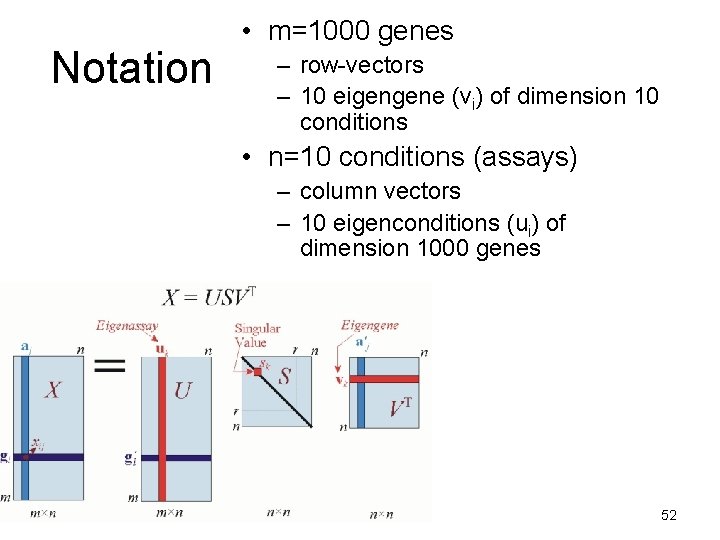
Notation • m=1000 genes – row-vectors – 10 eigengene (vi) of dimension 10 conditions • n=10 conditions (assays) – column vectors – 10 eigenconditions (ui) of dimension 1000 genes 52

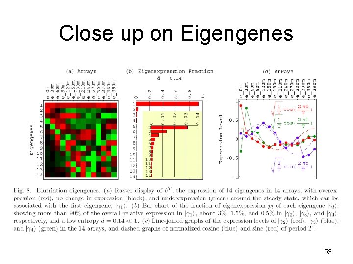
Close up on Eigengenes 53

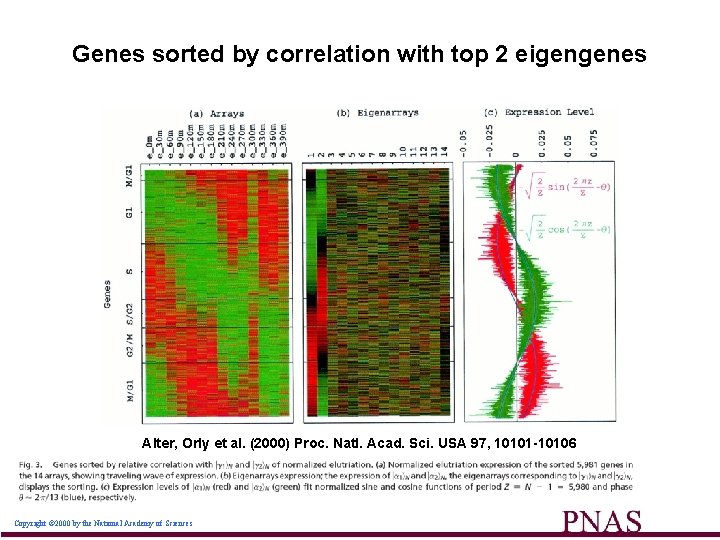
Genes sorted by correlation with top 2 eigengenes Alter, Orly et al. (2000) Proc. Natl. Acad. Sci. USA 97, 10101 -10106 Copyright © 2000 by the National Academy of Sciences 54

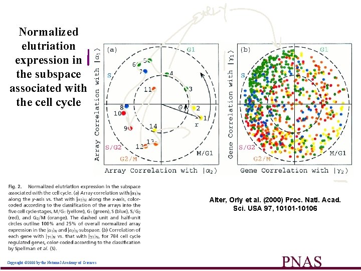
Normalized elutriation expression in the subspace associated with the cell cycle Alter, Orly et al. (2000) Proc. Natl. Acad. Sci. USA 97, 10101 -10106 Copyright © 2000 by the National Academy of Sciences 55

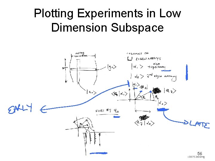
Plotting Experiments in Low Dimension Subspace 56 cbb 752 rd 0 mg

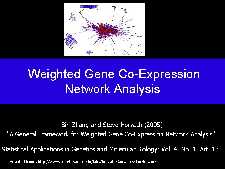
Weighted Gene Co-Expression Network Analysis Bin Zhang and Steve Horvath (2005) "A General Framework for Weighted Gene Co-Expression Network Analysis", Statistical Applications in Genetics and Molecular Biology: Vol. 4: No. 1, Art. 17. Adapted from : http: //www. genetics. ucla. edu/labs/horvath/Coexpression. Network

Module Detection • Numerous methods exist • Many methods define a suitable gene-gene dissimilarity measure and use clustering. • In our case: dissimilarity based on topological overlap • Clustering method: Average linkage hierarchical clustering – branches of the dendrogram are modules Adapted from : http: //www. genetics. ucla. edu/labs/horvath/Coexpression. Network

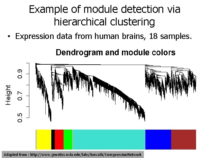
Example of module detection via hierarchical clustering • Expression data from human brains, 18 samples. Adapted from : http: //www. genetics. ucla. edu/labs/horvath/Coexpression. Network

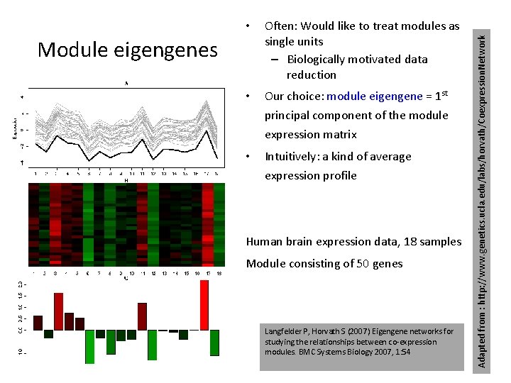
Often: Would like to treat modules as single units – Biologically motivated data reduction • Our choice: module eigengene = 1 st principal component of the module expression matrix • Intuitively: a kind of average expression profile Module eigengenes Human brain expression data, 18 samples Module consisting of 50 genes Langfelder P, Horvath S (2007) Eigengene networks for studying the relationships between co-expression modules. BMC Systems Biology 2007, 1: 54 Adapted from : http: //www. genetics. ucla. edu/labs/horvath/Coexpression. Network •

Unsupervised Mining Biplot

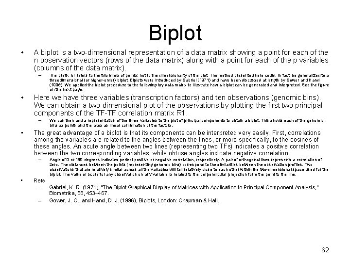
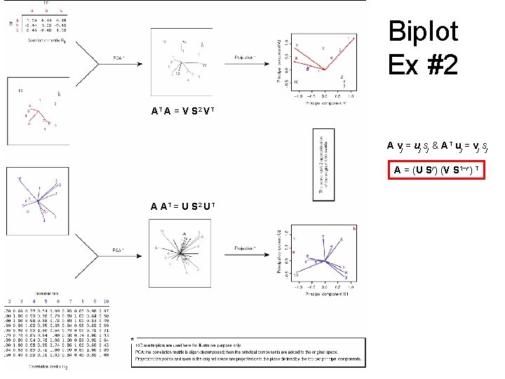
Biplot • A biplot is a two-dimensional representation of a data matrix showing a point for each of the n observation vectors (rows of the data matrix) along with a point for each of the p variables (columns of the data matrix). – • Here we have three variables (transcription factors) and ten observations (genomic bins). We can obtain a two-dimensional plot of the observations by plotting the first two principal components of the TF-TF correlation matrix R 1. – • We can then add a representation of the three variables to the plot of principal components to obtain a biplot. This shows each of the genomic bins as points and the axes as linear combination of the factors. The great advantage of a biplot is that its components can be interpreted very easily. First, correlations among the variables are related to the angles between the lines, or more specifically, to the cosines of these angles. An acute angle between two lines (representing two TFs) indicates a positive correlation between the two corresponding variables, while obtuse angles indicate negative correlation. – • The prefix ‘bi’ refers to the two kinds of points; not to the dimensionality of the plot. The method presented here could, in fact, be generalized to a threedimensional (or higher-order) biplot. Biplots were introduced by Gabriel (1971) and have been discussed at length by Gower and Hand (1996). We applied the biplot procedure to the following toy data matrix to illustrate how a biplot can be generated and interpreted. See the figure on the next page. Angle of 0 or 180 degrees indicates perfect positive or negative correlation, respectively. A pair of orthogonal lines represents a correlation of zero. The distances between the points (representing genomic bins) correspond to the similarities between the observation profiles. Two observations that are relatively similar across all the variables will fall relatively close to each other within the two-dimensional space used for the biplot. The value or score for any observation on any variable is related to the perpendicular projection form the point to the line. Refs – Gabriel, K. R. (1971), “The Biplot Graphical Display of Matrices with Application to Principal Component Analysis, ” Biometrika, 58, 453– 467. – Gower, J. C. , and Hand, D. J. (1996), Biplots, London: Chapman & Hall. 62

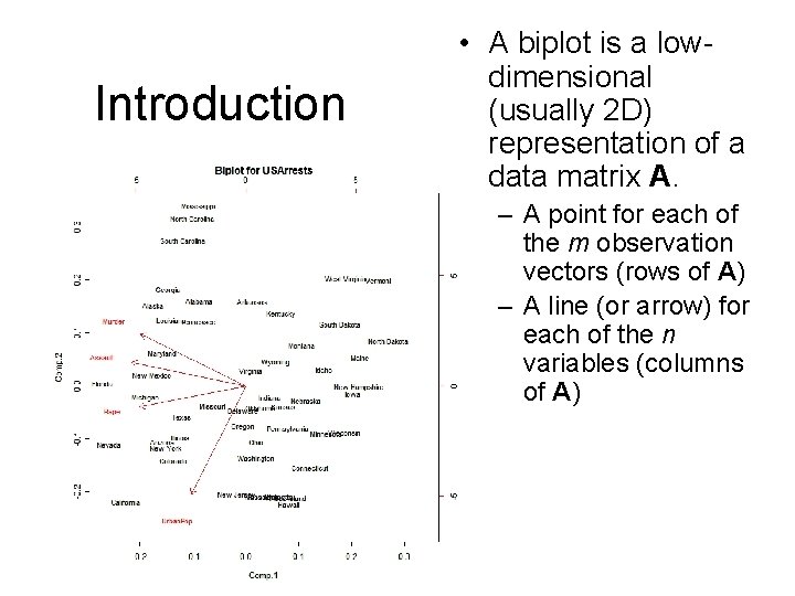
Introduction • A biplot is a lowdimensional (usually 2 D) representation of a data matrix A. – A point for each of the m observation vectors (rows of A) – A line (or arrow) for each of the n variables (columns of A)

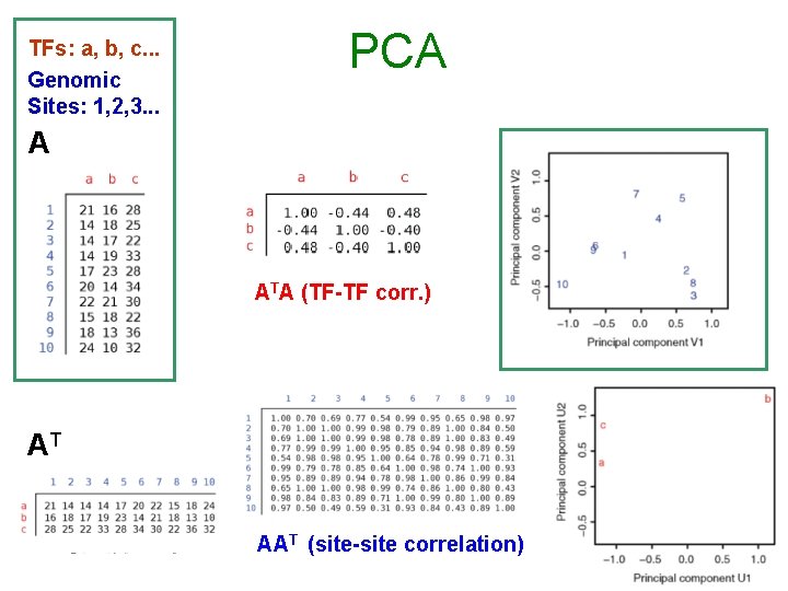
TFs: a, b, c. . . Genomic Sites: 1, 2, 3. . . PCA A ATA (TF-TF corr. ) AT AAT (site-site correlation)

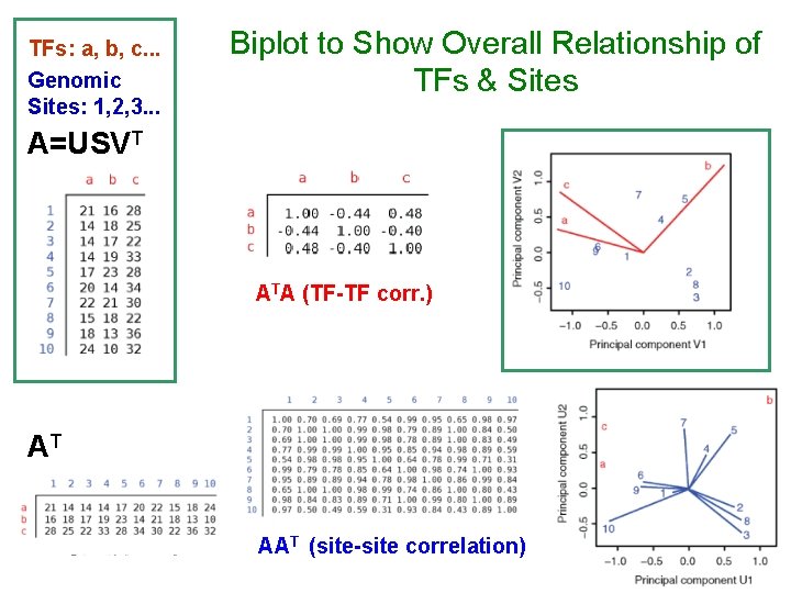
TFs: a, b, c. . . Genomic Sites: 1, 2, 3. . . Biplot to Show Overall Relationship of TFs & Sites A=USVT ATA (TF-TF corr. ) AT AAT (site-site correlation)

A’A A Biplot Ex

Biplot Ex #2 AT A = V S 2 V T A vj = uj sj & AT uj = vj sj A = (U Sr) (V S 1−r) T A A T = U S 2 UT

Biplot Ex #3 Assuming s=1, Av = u A Tu = v 68

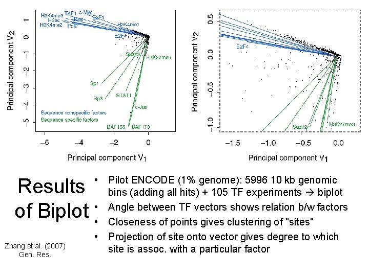
Results of Biplot Zhang et al. (2007) Gen. Res. • Pilot ENCODE (1% genome): 5996 10 kb genomic bins (adding all hits) + 105 TF experiments biplot • Angle between TF vectors shows relation b/w factors • Closeness of points gives clustering of "sites" • Projection of site onto vector gives degree to which site is assoc. with a particular factor

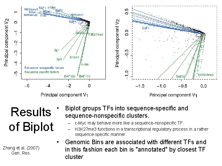
Results of Biplot Zhang et al. (2007) Gen. Res. • Biplot groups TFs into sequence-specific and sequence-nonspecific clusters. – c-Myc may behave more like a sequence-nonspecific TF. – H 3 K 27 me 3 functions in a transcriptional regulatory process in a rather sequence-specific manner. • Genomic Bins are associated with different TFs and in this fashion each bin is "annotated" by closest TF cluster

Unsupervised Mining CCA

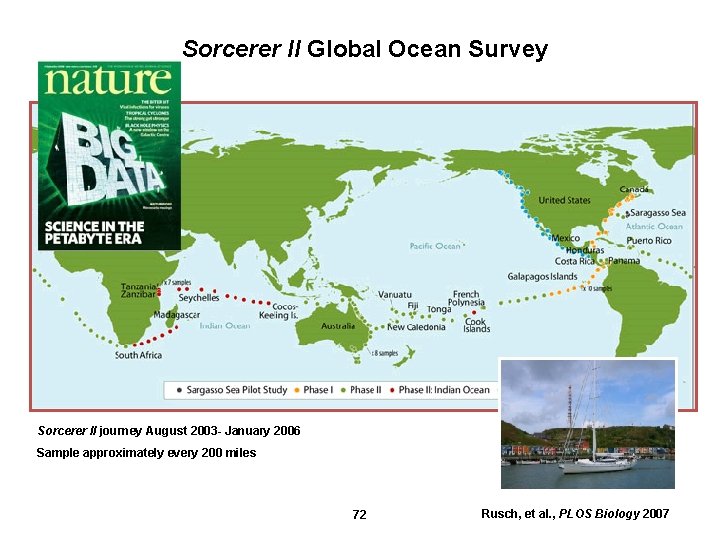
Sorcerer II Global Ocean Survey Sorcerer II journey August 2003 - January 2006 Sample approximately every 200 miles 72 Rusch, et al. , PLOS Biology 2007

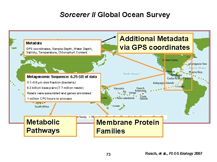
Sorcerer II Global Ocean Survey Additional Metadata via GPS coordinates Metadata GPS coordinates, Sample Depth, Water Depth, Salinity, Temperature, Chlorophyll Content Metagenomic Sequence: 6. 25 GB of data 0. 1– 0. 8 μm size fraction (bacteria) 6. 3 billion base pairs (7. 7 million reads) Reads were assembled and genes annotated 1 million CPU hours to process Metabolic Pathways Membrane Protein Families 73 Rusch, et al. , PLOS Biology 2007

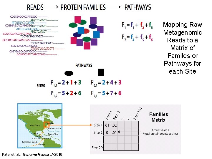
Mapping Raw Metagenomic Reads to a Matrix of Familes or Pathways for each Site Families Matrix Patel et. al. , Genome Research 2010

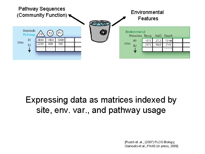
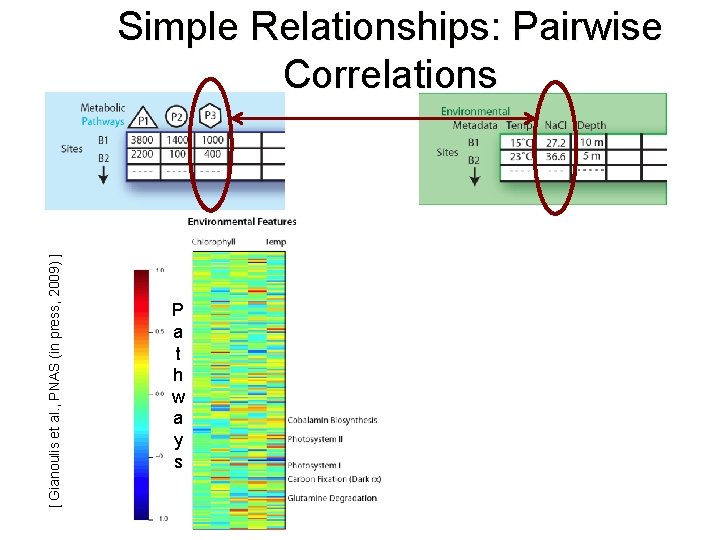
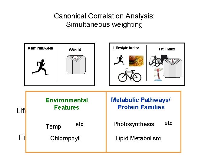
Pathway Sequences (Community Function) Environmental Features Expressing data as matrices indexed by site, env. var. , and pathway usage [Rusch et. al. , (2007) PLOS Biology; Gianoulis et al. , PNAS (in press, 2009]

[ Gianoulis et al. , PNAS (in press, 2009) ] Simple Relationships: Pairwise Correlations P a t h w a y s

Canonical Correlation Analysis: Simultaneous weighting # km run/week Lifestyle Index Weight Lifestyle Index = a Fit Index = a +b +b Fit Index +c +c

Canonical Correlation Analysis: Simultaneous weighting # km run/week Lifestyle Index Weight Metabolic Pathways/ Protein Families Environmental Features Lifestyle Index = a Temp +b +c Photosynthesis etc Fit Index Chlorophyll = a Fit Index +b Lipid+c Metabolism etc

CCA: Finding Variables with Large Projections in "Correlation Circle" The goal of this technique is to interpret cross-variance matrices We do this by defining a change of basis. Gianoulis et al. , PNAS 2009

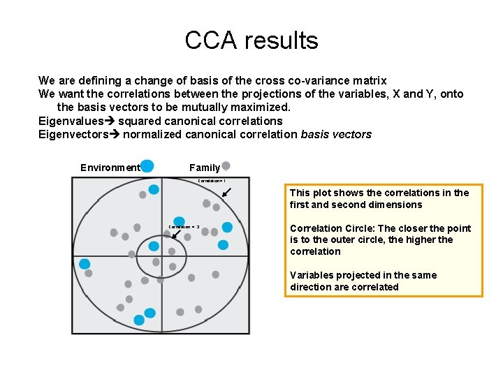
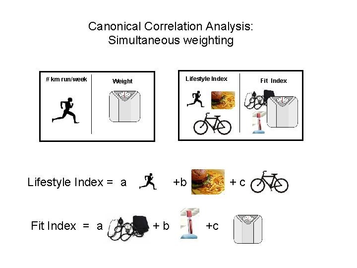
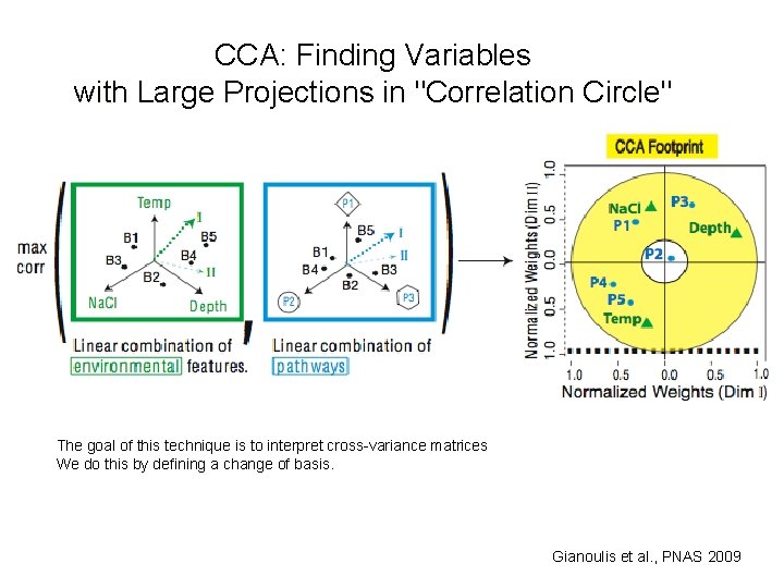
CCA results We are defining a change of basis of the cross co-variance matrix We want the correlations between the projections of the variables, X and Y, onto the basis vectors to be mutually maximized. Eigenvalues squared canonical correlations Eigenvectors normalized canonical correlation basis vectors Environment Family Correlation= 1 This plot shows the correlations in the first and second dimensions Correlation =. 3 Correlation Circle: The closer the point is to the outer circle, the higher the correlation Variables projected in the same direction are correlated

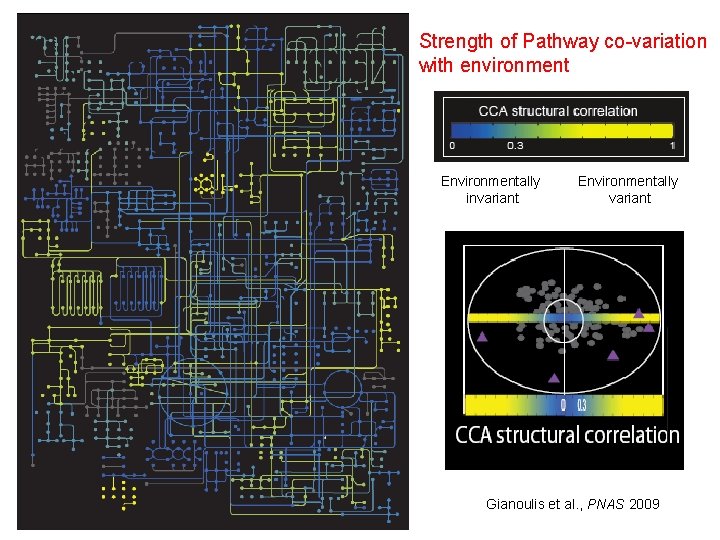
Strength of Pathway co-variation with environment Circuit Map Environmentally invariant Environmentally variant Gianoulis et al. , PNAS 2009

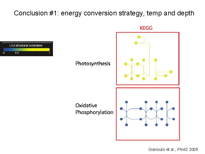
Conclusion #1: energy conversion strategy, temp and depth Gianoulis et al. , PNAS 2009