Bioinformatics GBIO 0009 1 Biological Sequences Comparison GBIO

Bioinformatics GBIO 0009 1 Biological Sequences Comparison GBIO 0009 -1 Presented by Kirill Bessonov Oct 27, 2015 __________________________________________________________ Kirill Bessonov slide 1

Bioinformatics GBIO 0009 1 Biological Sequences Lecture structure 1. 2. 3. 4. Introduction Global Alignment: Needleman Wunsch Local Alignment: Smith Waterman Illustrations – Sequences identification via BLAST – Retrieval of sequences via Uni. Prot and R – Alignment of sequences via R (seqinr) – Detection of ORFs with R – Comparing genomes of two species __________________________________________________________ Kirill Bessonov slide 2

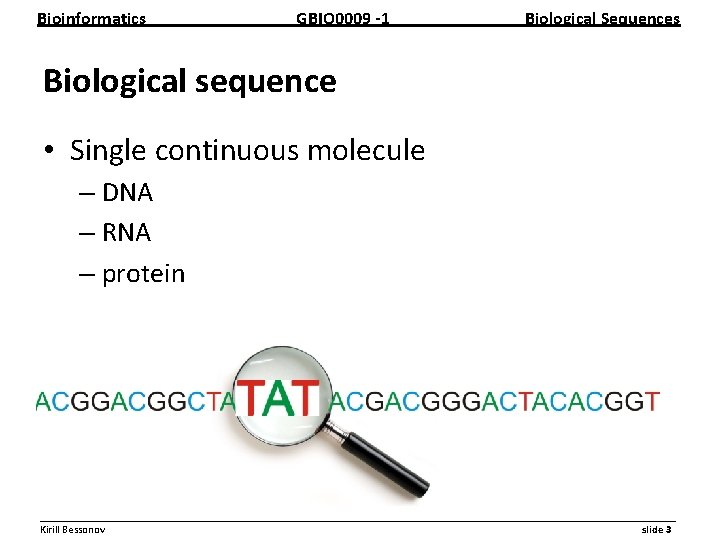
Bioinformatics GBIO 0009 1 Biological Sequences Biological sequence • Single continuous molecule – DNA – RNA – protein __________________________________________________________ Kirill Bessonov slide 3

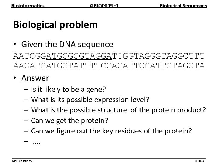
Bioinformatics GBIO 0009 1 Biological Sequences Biological problem • Given the DNA sequence AATCGGATGCGCGTAGGATCGGTAGGCTTT AAGATCATGCTATTTTCGAGATTCTAGCTA • Answer – Is it likely to be a gene? – What is its possible expression level? – What is the possible structure of the protein product? – Can we get the protein? – Can we figure out the key residues of the protein? – …. __________________________________________________________ Kirill Bessonov slide 4

Bioinformatics GBIO 0009 1 Biological Sequences Alphabet – In the case of DNA • A, C, T, G – In the case of RNA • A, C, U, G – In the case of protein • 20 amino acids • Complete list is found here __________________________________________________________ Kirill Bessonov slide 5

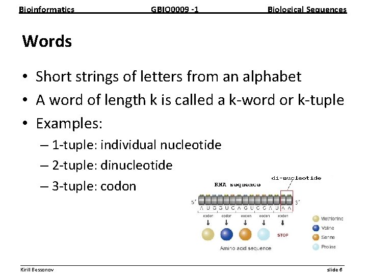
Bioinformatics GBIO 0009 1 Biological Sequences Words • Short strings of letters from an alphabet • A word of length k is called a k word or k tuple • Examples: – 1 tuple: individual nucleotide – 2 tuple: dinucleotide – 3 tuple: codon __________________________________________________________ Kirill Bessonov slide 6

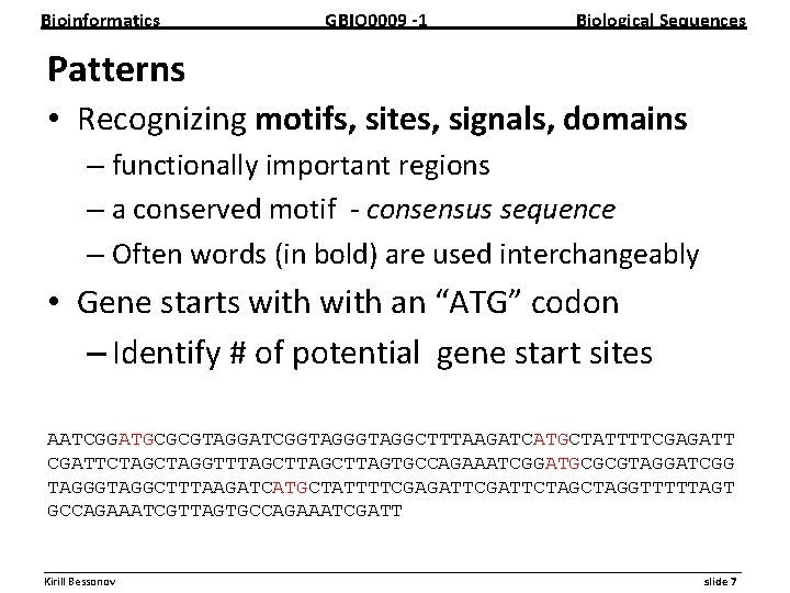
Bioinformatics GBIO 0009 1 Biological Sequences Patterns • Recognizing motifs, sites, signals, domains – functionally important regions – a conserved motif consensus sequence – Often words (in bold) are used interchangeably • Gene starts with an “ATG” codon – Identify # of potential gene start sites AATCGGATGCGCGTAGGATCGGTAGGCTTTAAGATCATGCTATTTTCGAGATT CGATTCTAGGTTTAGCTTAGTGCCAGAAATCGGATGCGCGTAGGATCGG TAGGGTAGGCTTTAAGATCATGCTATTTTCGAGATTCTAGCTAGGTTTTTAGT GCCAGAAATCGTTAGTGCCAGAAATCGATT __________________________________________________________ Kirill Bessonov slide 7

Bioinformatics GBIO 0009 1 Biological Sequences Probability • What is the probability distribution of the number of times a given base N (A, C, T or G) occurs in a random DNA sequence of length Ln? – Assume X 1, …, Xn is the sequence of Ln – Count the number of times N appears – Calculate probabilities • P(Xi=N) = # {Xi=N}/ Ln • P(Xi= not N) = 1 – p. N Ex: Given ATCCTACTGT Ln = 10 – P(Xi=A) = 2/10 = 0. 2 – P(Xi=T or C or G) = 1 – 0. 2 = 0. 8 __________________________________________________________ Kirill Bessonov slide 8

Bioinformatics GBIO 0009 1 Biological Sequences Alignments __________________________________________________________ Kirill Bessonov slide 9

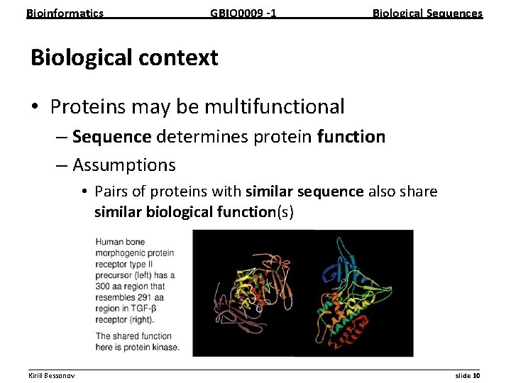
Bioinformatics GBIO 0009 1 Biological Sequences Biological context • Proteins may be multifunctional – Sequence determines protein function – Assumptions • Pairs of proteins with similar sequence also share similar biological function(s) __________________________________________________________ Kirill Bessonov slide 10

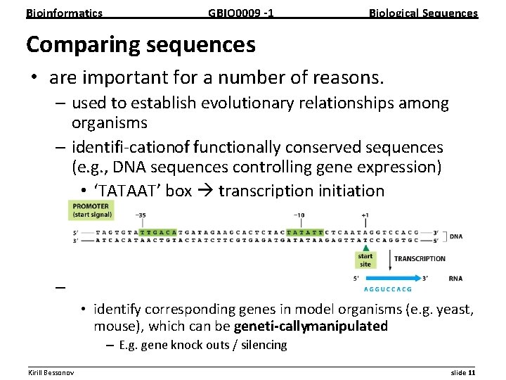
Bioinformatics GBIO 0009 1 Biological Sequences Comparing sequences • are important for a number of reasons. – used to establish evolutionary relationships among organisms – identifi cationof functionally conserved sequences (e. g. , DNA sequences controlling gene expression) • ‘TATAAT’ box transcription initiation – develop models for human diseases • identify corresponding genes in model organisms (e. g. yeast, mouse), which can be geneti callymanipulated – E. g. gene knock outs / silencing __________________________________________________________ Kirill Bessonov slide 11

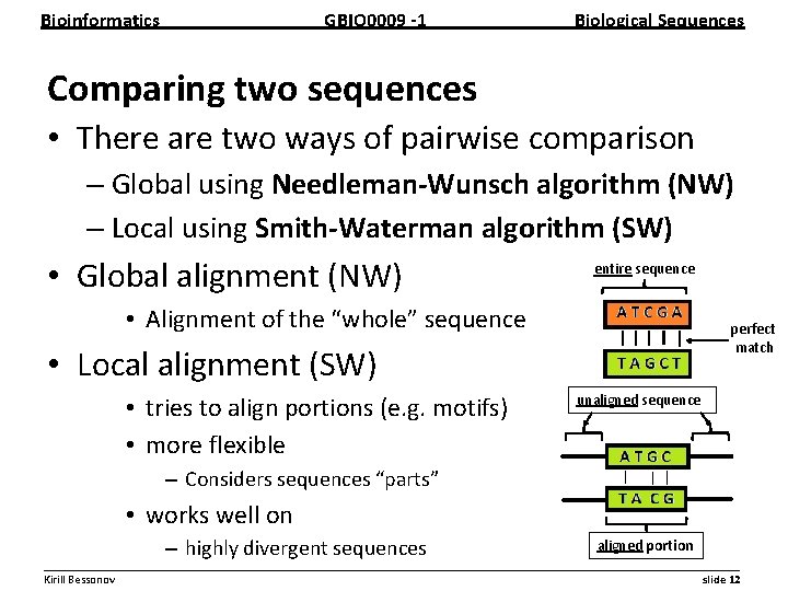
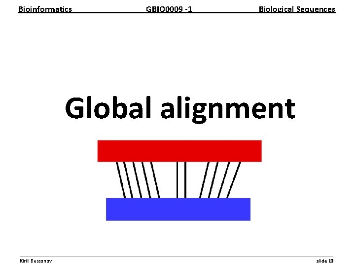
Bioinformatics GBIO 0009 1 Biological Sequences Comparing two sequences • There are two ways of pairwise comparison – Global using Needleman Wunsch algorithm (NW) – Local using Smith Waterman algorithm (SW) • Global alignment (NW) entire sequence • Alignment of the “whole” sequence perfect match • Local alignment (SW) • tries to align portions (e. g. motifs) • more flexible unaligned sequence – Considers sequences “parts” • works well on – highly divergent sequences aligned portion __________________________________________________________ Kirill Bessonov slide 12

Bioinformatics GBIO 0009 1 Biological Sequences Global alignment __________________________________________________________ Kirill Bessonov slide 13

Bioinformatics GBIO 0009 1 Biological Sequences Global alignment (NW) • Sequences are aligned end to end along their entire length • Many possible alignments are produced – The alignment with the highest score is chosen • Naïve algorithm is very inefficient (Oexp) – To align sequence of length 15, need to consider • (insertion, deletion, gap)15 = 315 = 1, 4*107 – Impractical for sequences of length >20 nt • Used to analyze homology/similarity of – genes and proteins – between species __________________________________________________________ Kirill Bessonov slide 14

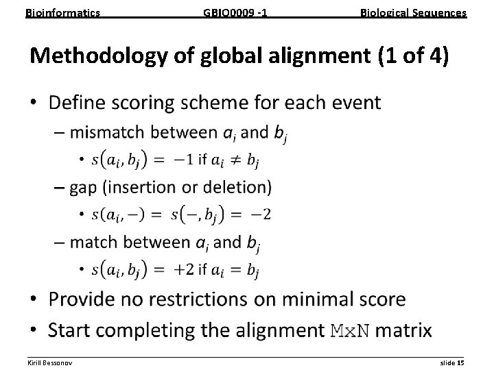
Bioinformatics GBIO 0009 1 Biological Sequences Methodology of global alignment (1 of 4) • __________________________________________________________ Kirill Bessonov slide 15

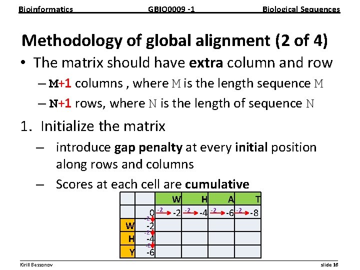
Bioinformatics GBIO 0009 1 Biological Sequences Methodology of global alignment (2 of 4) • The matrix should have extra column and row – M+1 columns , where M is the length sequence M – N+1 rows, where N is the length of sequence N 1. Initialize the matrix – introduce gap penalty at every initial position along rows and columns – Scores at each cell are cumulative W 2 H 4 A T 6 2 8 2 2 2 0 2 W 2 2 H 4 2 Y 6 __________________________________________________________ Kirill Bessonov slide 16

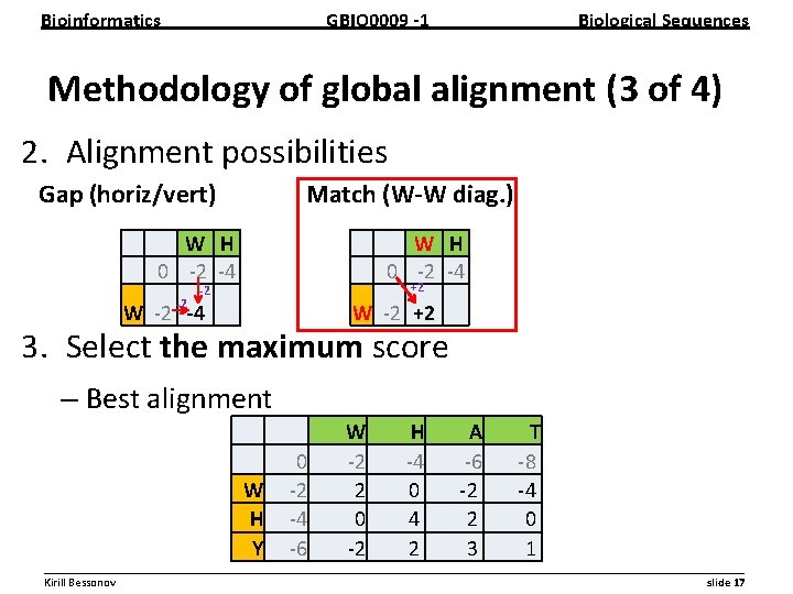
Bioinformatics GBIO 0009 1 Biological Sequences Methodology of global alignment (3 of 4) 2. Alignment possibilities Gap (horiz/vert) Match (W W diag. ) W H 0 2 4 2 W H 0 2 4 +2 2 W 2 4 W 2 +2 3. Select the maximum score – Best alignment W H Y 0 2 4 6 W 2 2 0 2 H 4 0 4 2 A 6 2 2 3 T 8 4 0 1 __________________________________________________________ Kirill Bessonov slide 17

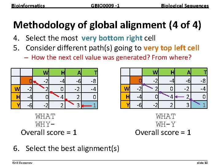
Bioinformatics GBIO 0009 1 Biological Sequences Methodology of global alignment (4 of 4) 4. Select the most very bottom right cell 5. Consider different path(s) going to very top left cell – How the next cell value was generated? From where? W H Y 0 2 4 6 W 2 2 0 2 H 4 0 4 2 A 6 2 2 3 T 8 4 0 1 WHAT WHYOverall score = 1 W H Y 0 2 4 6 W 2 2 0 2 H 4 0 4 2 A 6 2 2 3 T 8 4 0 1 WHAT WH-Y Overall score = 1 6. Select the best alignment(s) __________________________________________________________ Kirill Bessonov slide 18

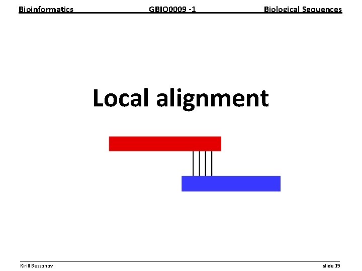
Bioinformatics GBIO 0009 1 Biological Sequences Local alignment __________________________________________________________ Kirill Bessonov slide 19

Bioinformatics GBIO 0009 1 Biological Sequences Local alignment (SW) • Sequences are aligned to find regions where the best alignment occurs (i. e. highest score) • Assumes a local context (aligning parts of seq. ) • Ideal for finding short motifs, DNA binding sites – helix loop helix (b. HLH) motif – TATAAT box (a famous promoter region) – DNA binding site • Works well on highly divergent sequences __________________________________________________________ Kirill Bessonov slide 20

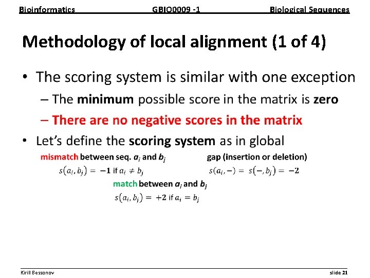
Bioinformatics GBIO 0009 1 Biological Sequences Methodology of local alignment (1 of 4) • __________________________________________________________ Kirill Bessonov slide 21

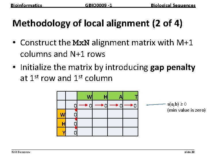
Bioinformatics GBIO 0009 1 Biological Sequences Methodology of local alignment (2 of 4) • Construct the Mx. N alignment matrix with M+1 columns and N+1 rows • Initialize the matrix by introducing gap penalty at 1 st row and 1 st column 0 W 0 H 0 Y 0 W H A T 0 0 s(a, b) ≥ 0 (min value is zero) __________________________________________________________ Kirill Bessonov slide 22

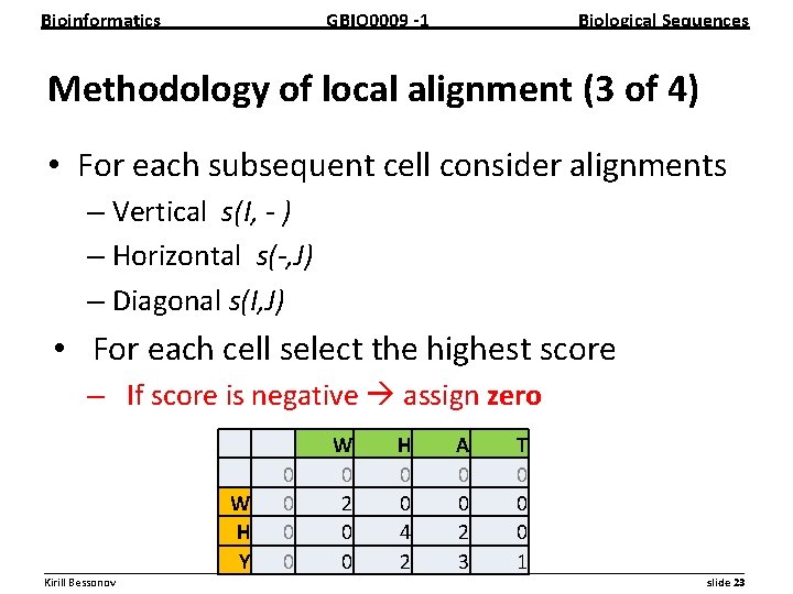
Bioinformatics GBIO 0009 1 Biological Sequences Methodology of local alignment (3 of 4) • For each subsequent cell consider alignments – Vertical s(I, - ) – Horizontal s(-, J) – Diagonal s(I, J) • For each cell select the highest score – If score is negative assign zero W H A T 0 0 0 W 0 2 0 0 0 H 0 0 4 2 0 Y 0 0 2 3 1 __________________________________________________________ Kirill Bessonov slide 23

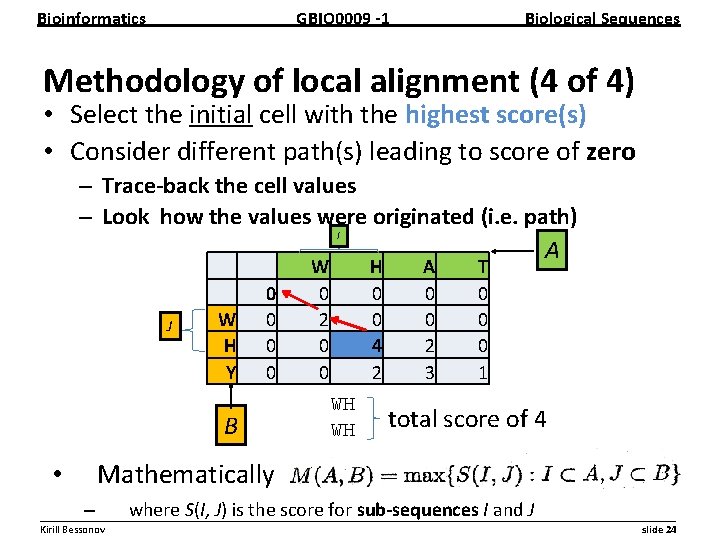
Bioinformatics GBIO 0009 1 Biological Sequences Methodology of local alignment (4 of 4) • Select the initial cell with the highest score(s) • Consider different path(s) leading to score of zero – Trace back the cell values – Look how the values were originated (i. e. path) I J W H Y 0 0 B W 0 2 0 0 H 0 0 4 2 WH WH A 0 0 2 3 T 0 0 0 1 A total score of 4 Mathematically • – where S(I, J) is the score for sub sequences I and J __________________________________________________________ Kirill Bessonov slide 24

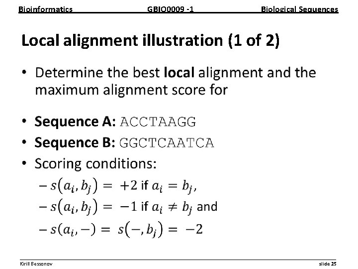
Bioinformatics GBIO 0009 1 Biological Sequences Local alignment illustration (1 of 2) • __________________________________________________________ Kirill Bessonov slide 25

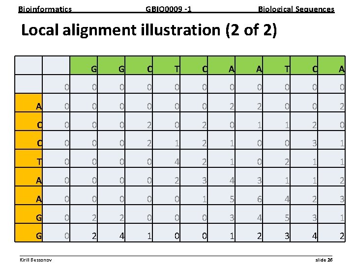
Bioinformatics GBIO 0009 1 Biological Sequences Local alignment illustration (2 of 2) G G C T C A A T C A 0 0 0 A 0 0 0 0 2 2 0 0 2 C 0 0 0 2 0 1 1 2 0 C 0 0 0 2 1 0 0 2 3 1 T 0 0 4 2 1 0 2 0 1 1 A 0 0 2 3 4 3 1 1 2 A 0 0 0 1 5 6 4 2 3 G 0 2 2 0 0 0 3 4 5 3 1 G 0 2 4 1 0 0 1 2 3 4 2 __________________________________________________________ Kirill Bessonov slide 26

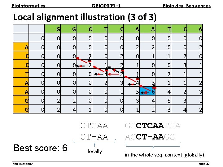
Bioinformatics GBIO 0009 1 Biological Sequences Local alignment illustration (3 of 3) A C C T A A G G 0 0 0 0 0 G 0 0 0 0 2 2 G 0 0 0 0 2 4 C 0 0 2 2 0 0 1 T 0 0 0 1 4 2 0 0 0 CTCAA CT-AA Best score: 6 locally C 0 0 2 2 2 3 1 0 0 A 0 2 0 1 1 4 5 3 1 A 0 2 1 0 0 3 6 4 2 T 0 0 1 0 2 1 4 5 3 C 0 0 2 3 1 1 2 3 4 A 0 2 0 1 1 2 3 1 2 GGCTCAATCA ACCT-AAGG in the whole seq. context (globally) __________________________________________________________ Kirill Bessonov slide 27

Bioinformatics GBIO 0009 1 Biological Sequences Aligning proteins Globally and Locally __________________________________________________________ Kirill Bessonov slide 28

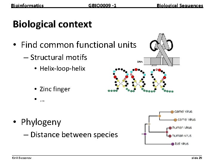
Bioinformatics GBIO 0009 1 Biological Sequences Biological context • Find common functional units – Structural motifs • Helix loop helix • Zinc finger • … • Phylogeny – Distance between species __________________________________________________________ Kirill Bessonov slide 29

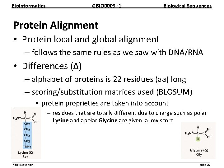
Bioinformatics GBIO 0009 1 Biological Sequences Protein Alignment • Protein local and global alignment – follows the same rules as we saw with DNA/RNA • Differences (∆) – alphabet of proteins is 22 residues (aa) long – scoring/substitution matrices used (BLOSUM) • protein proprieties are taken into account – residues that are totally different due to charge such as polar Lysine and apolar Glycine are given a low score __________________________________________________________ Kirill Bessonov slide 30

Bioinformatics GBIO 0009 1 Biological Sequences Substitution matrices • Protein sequences are more complex – matrices = collection of scoring rules • Matrices over events such as – mismatch and perfect match • Need to define gap penalty separately • E. g. BLOcks SUbstitution Matrix (BLOSUM) __________________________________________________________ Kirill Bessonov slide 31

Bioinformatics GBIO 0009 1 Biological Sequences BLOSUM x matrices • Constructed from aligned sequences with specific x% similarity – matrix built using sequences with no more then 50% similarity is called BLOSUM 50 • For highly mutating / dissimilar sequences use – BLOSUM 45 and lower • For highly conserved / similar sequences use – BLOSUM 62 and higher __________________________________________________________ Kirill Bessonov slide 32

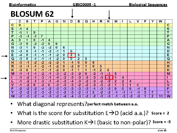
Bioinformatics GBIO 0009 1 Biological Sequences BLOSUM 62 • What diagonal represents? perfect match between a. a. • What is the score for substitution E D (acid a. a. )? Score = 2 • More drastic substitution K I (basic to non polar)? Score = 3 __________________________________________________________ Kirill Bessonov slide 33

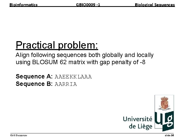
Bioinformatics GBIO 0009 1 Biological Sequences Practical problem: Align following sequences both globally and locally using BLOSUM 62 matrix with gap penalty of -8 Sequence A: AAEEKKLAAA Sequence B: AARRIA __________________________________________________________ Kirill Bessonov slide 34

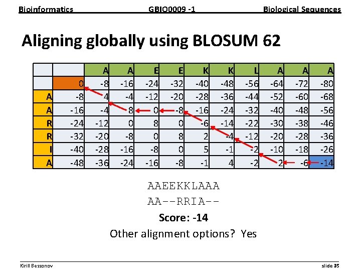
Bioinformatics GBIO 0009 1 Biological Sequences Aligning globally using BLOSUM 62 A A R R I A 0 8 16 24 32 40 48 A 8 4 4 12 20 28 36 A 16 4 8 0 8 16 24 E 24 12 0 8 16 E 32 20 8 0 8 K 40 28 16 6 2 5 1 K 48 36 24 14 4 1 4 L 56 44 32 22 12 2 2 A 64 52 40 30 20 10 2 A 72 60 48 38 28 18 6 A 80 68 56 46 36 26 14 AAEEKKLAAA AA--RRIA-Score: 14 Other alignment options? Yes __________________________________________________________ Kirill Bessonov slide 35

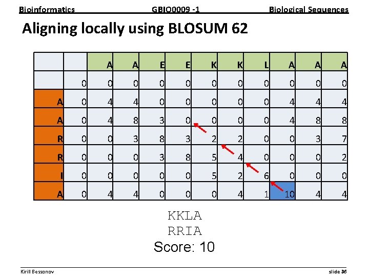
Bioinformatics GBIO 0009 1 Biological Sequences Aligning locally using BLOSUM 62 A A E E K K L A A A 0 0 0 A 0 4 4 0 0 0 4 4 4 A 0 4 8 3 0 0 4 8 8 R 0 0 3 8 3 2 2 0 0 3 7 R 0 0 0 3 8 5 4 0 0 0 2 I 0 0 0 5 2 6 0 0 0 A 0 4 4 0 0 0 4 1 10 4 4 KKLA RRIA Score: 10 __________________________________________________________ Kirill Bessonov slide 36

Bioinformatics GBIO 0009 1 Biological Sequences Practical 1 of 5: Using BLAST for sequence identification __________________________________________________________ Kirill Bessonov slide 37

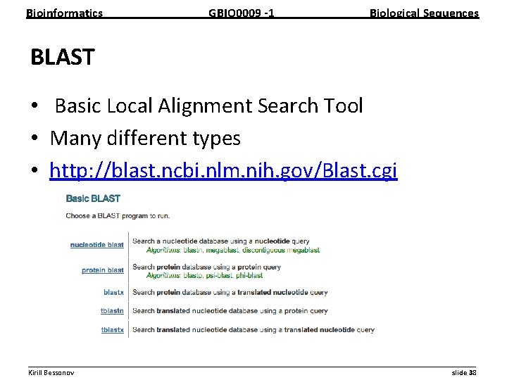
Bioinformatics GBIO 0009 1 Biological Sequences BLAST • Basic Local Alignment Search Tool • Many different types • http: //blast. ncbi. nlm. nih. gov/Blast. cgi __________________________________________________________ Kirill Bessonov slide 38

Bioinformatics GBIO 0009 1 Biological Sequences Types • blastn – nucleotide query vs nucleotide database • blastp – protein query vs protein DB • blastx – translated in 6 frames nucleotide query vs protein DB __________________________________________________________ Kirill Bessonov slide 39

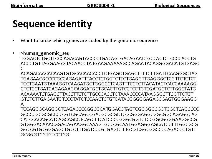
Bioinformatics GBIO 0009 1 Biological Sequences Sequence identity • Want to know which genes are coded by the genomic sequence • >human_genomic_seq TGGACTCTGCTTCCCAGACAGTACCCCTGACAGAACTGCCACTCTCCCCACCTG ACCCTGTTAGGAAGGTACAACCTATGAAGAAAAAGCCAGAATACAGGGGACATGTGAGC C ACAGACAACACAAGTGTGCACAACACCTCTGAGCTTTTCTTGATTCAAGGGCTAG TGAGAACGCCCCGCCAGAGATTTACCTCTGGTCTTCTGAGGTTGAGGGCTCGTTCTCTCT TCCTGAATGTAAAGGTCAAGATGCTGGGCCTCAGTTTCCTCTTACATACTCACCAAAAGG CTCTCCTGATCAGAGAAGCAGGATGCTGCACTTGTCCTCCTGTCGATGCTCTTGGCTATG ACAAAATCTGAGCTTACCTTCTCTTGCCCACCTCTAAACCCCATAAGGGCTTCGTTCTGT GTCTCTTGAGAATGTCCCTATCTCCAACTCTGTCATACGGGGGAGAGCGAGTGGGAAGG A TCCAGGGCTCAGACCCCGGCGCATGGACCTAGTCGGGGGCGCTGGCTCAGCCCCGCGCGCCCCCGTCGCAGCCGACGCGCGCTCCCGGGAGGCGGCGGCAGAGGCAG CATCCACAGCATCAGCAGCCTCAGCTTCATCCCCGGGCGGTCTCCGGCGGGGAAGGCCG GTGGGACAAACGGACAGAAGGCAAAGTGCCCGCAATGGAGCATCCTTTGGCGCG GGCCGTGCGGGAGCTGCCTTTGATCCCGTGAGCTTTGCGCGGCGGCCCCAGACCCTGTT GCGGGTCGTGTCCTGG __________________________________________________________ Kirill Bessonov slide 40

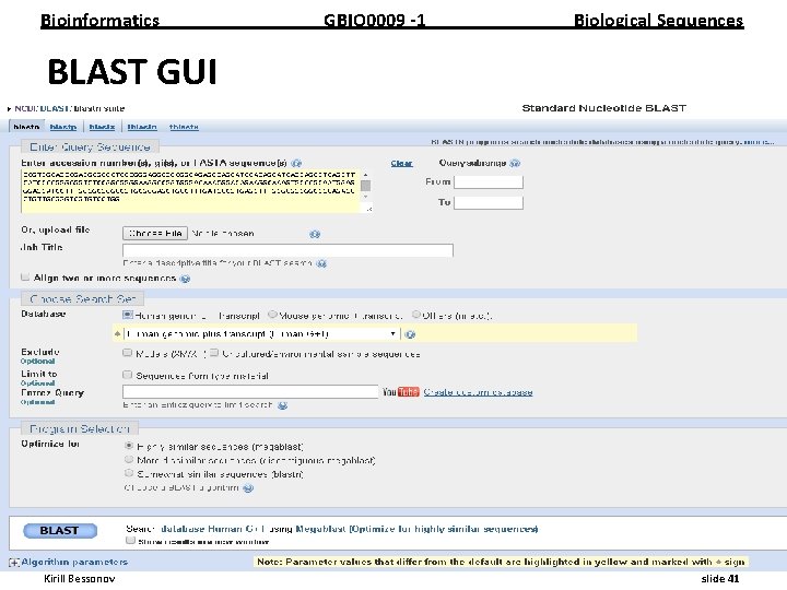
Bioinformatics GBIO 0009 1 Biological Sequences BLAST GUI __________________________________________________________ Kirill Bessonov slide 41

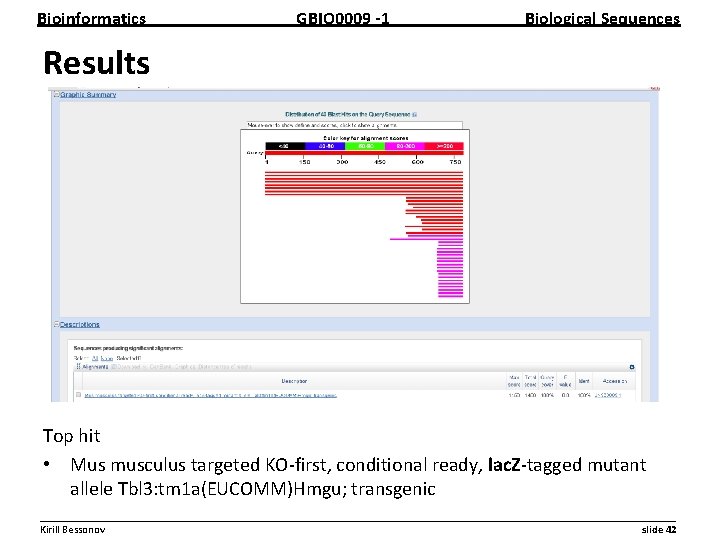
Bioinformatics GBIO 0009 1 Biological Sequences Results Top hit • Mus musculus targeted KO first, conditional ready, lac. Z tagged mutant allele Tbl 3: tm 1 a(EUCOMM)Hmgu; transgenic __________________________________________________________ Kirill Bessonov slide 42

Bioinformatics GBIO 0009 1 Biological Sequences Practical 2 of 5 : Sequence Retrieval and Analysis via R (seqinr) __________________________________________________________ Kirill Bessonov slide 43

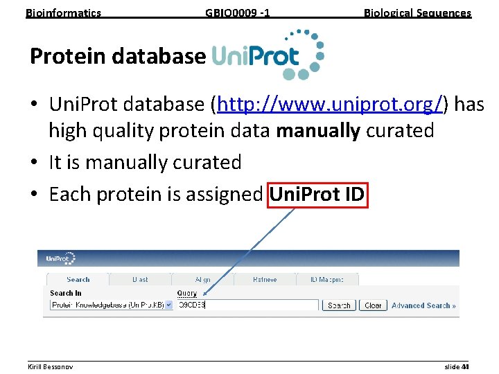
Bioinformatics GBIO 0009 1 Biological Sequences Protein database • Uni. Prot database (http: //www. uniprot. org/) has high quality protein data manually curated • It is manually curated • Each protein is assigned Uni. Prot ID __________________________________________________________ Kirill Bessonov slide 44

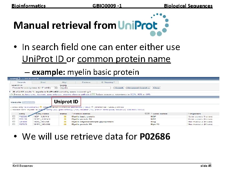
Bioinformatics GBIO 0009 1 Biological Sequences Manual retrieval from • In search field one can enter either use Uni. Prot ID or common protein name – example: myelin basic protein Uniprot ID • We will use retrieve data for P 02686 __________________________________________________________ Kirill Bessonov slide 45

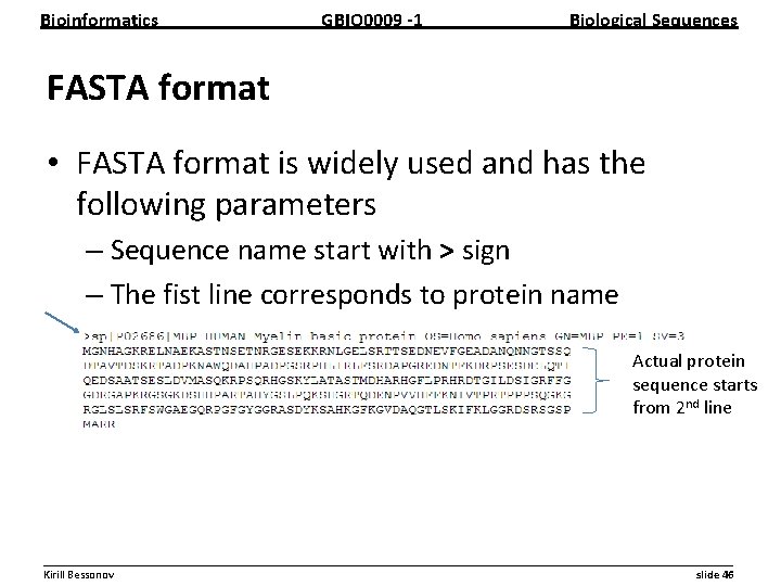
Bioinformatics GBIO 0009 1 Biological Sequences FASTA format • FASTA format is widely used and has the following parameters – Sequence name start with > sign – The fist line corresponds to protein name Actual protein sequence starts from 2 nd line __________________________________________________________ Kirill Bessonov slide 46

Bioinformatics GBIO 0009 1 Biological Sequences Retrieving protein data with R and Seqin. R • Can “talk” programmatically to Uni. Prot database using R and seqin. R library – seqin. R library is suitable for • “Biological Sequences Retrieval and Analysis” • Detailed manual could be found here – Install this library in your R environment install. packages("seqinr") library("seqinr") – Choose database to retrieve data from choosebank("swissprot") – Download data object for target protein (P 02686) MBP_HUMAN = query("MBP_HUMAN", "AC=P 02686") – See sequence of the object MBP_HUMAN_seq = get. Sequence(MBP_HUMAN); MBP_HUMAN_seq __________________________________________________________ Kirill Bessonov slide 47

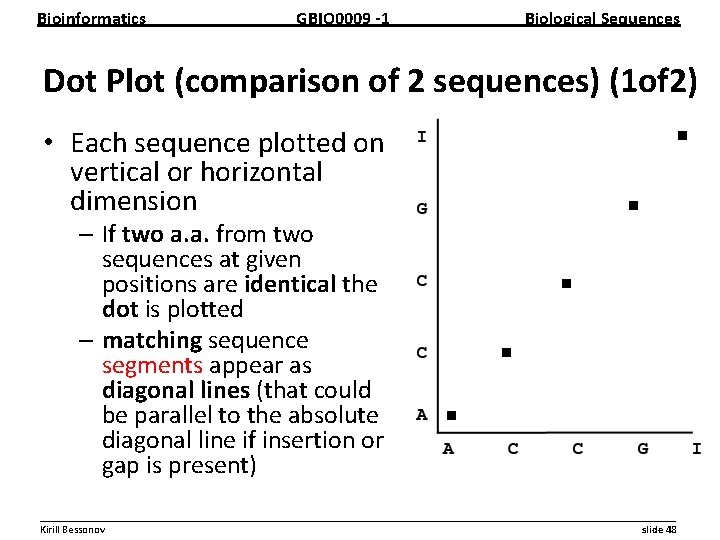
Bioinformatics GBIO 0009 1 Biological Sequences Dot Plot (comparison of 2 sequences) (1 of 2) • Each sequence plotted on vertical or horizontal dimension – If two a. a. from two sequences at given positions are identical the dot is plotted – matching sequence segments appear as diagonal lines (that could be parallel to the absolute diagonal line if insertion or gap is present) __________________________________________________________ Kirill Bessonov slide 48

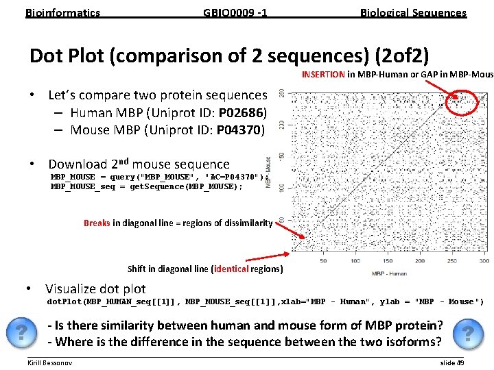
Bioinformatics GBIO 0009 1 Biological Sequences Dot Plot (comparison of 2 sequences) (2 of 2) INSERTION in MBP Human or GAP in MBP Mous • Let’s compare two protein sequences – Human MBP (Uniprot ID: P 02686) – Mouse MBP (Uniprot ID: P 04370) • Download 2 nd mouse sequence MBP_MOUSE = query("MBP_MOUSE", "AC=P 04370"); MBP_MOUSE_seq = get. Sequence(MBP_MOUSE); Breaks in diagonal line = regions of dissimilarity Shift in diagonal line (identical regions) • Visualize dot plot dot. Plot(MBP_HUMAN_seq[[1]], MBP_MOUSE_seq[[1 ]], xlab="MBP - Human", ylab = "MBP - Mouse ") Is there similarity between human and mouse form of MBP protein? Where is the difference in the sequence between the two isoforms? __________________________________________________________ Kirill Bessonov slide 49

Bioinformatics GBIO 0009 1 Biological Sequences Practical 3 of 5: Pairwise global and local alignments via R and Biostrings __________________________________________________________ Kirill Bessonov slide 50

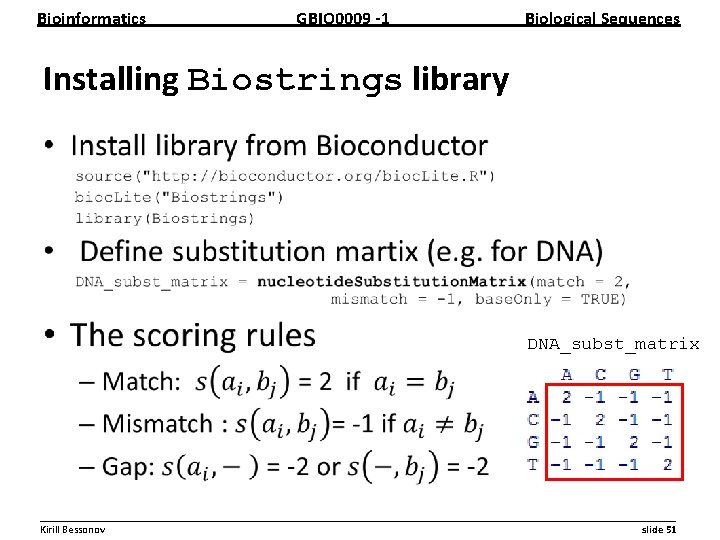
Bioinformatics GBIO 0009 1 Biological Sequences Installing Biostrings library • DNA_subst_matrix __________________________________________________________ Kirill Bessonov slide 51

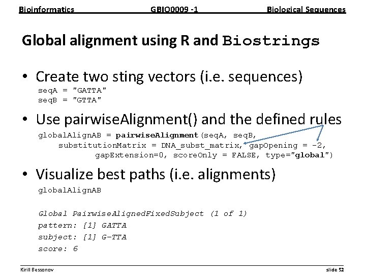
Bioinformatics GBIO 0009 1 Biological Sequences Global alignment using R and Biostrings • Create two sting vectors (i. e. sequences) seq. A = "GATTA" seq. B = "GTTA" • Use pairwise. Alignment() and the defined rules global. Align. AB = pairwise. Alignment(seq. A, seq. B, substitution. Matrix = DNA_subst_matrix, gap. Opening = -2, gap. Extension=0, score. Only = FALSE, type="global") • Visualize best paths (i. e. alignments) global. Align. AB Global Pairwise. Aligned. Fixed. Subject (1 of 1) pattern: [1] GATTA subject: [1] G-TTA score: 6 __________________________________________________________ Kirill Bessonov slide 52

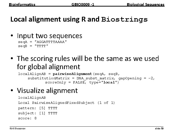
Bioinformatics GBIO 0009 1 Biological Sequences Local alignment using R and Biostrings • Input two sequences seq. A = "AGGATTTTAAAA" seq. B = "TTTT" • The scoring rules will be the same as we used for global alignment local. Align. AB = pairwise. Alignment(seq. A, seq. B, substitution. Matrix = DNA_subst_matrix, gap. Opening = -2, score. Only = FALSE, type="local") • Visualize alignment local. Align. AB Local Pairwise. Aligned. Fixed. Subject (1 of 1) pattern: [5] TTTT subject: [1] TTTT score: 8 __________________________________________________________ Kirill Bessonov slide 53

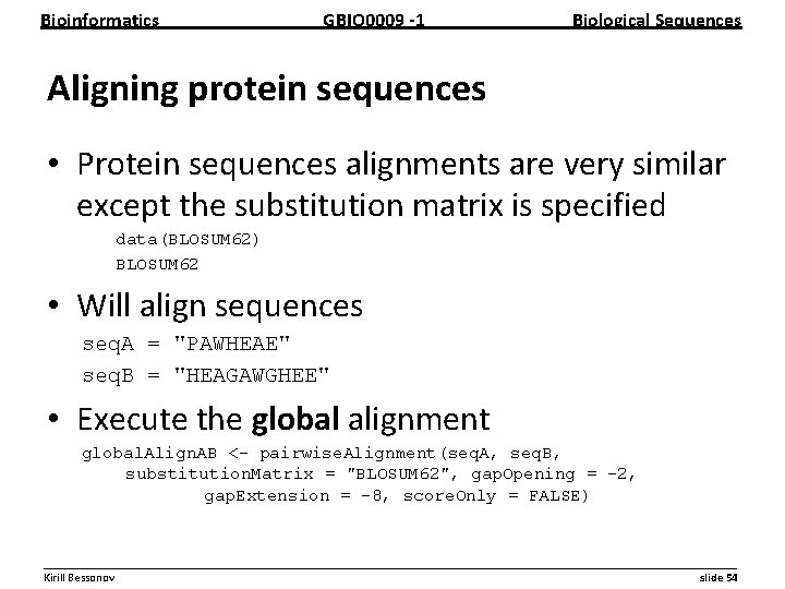
Bioinformatics GBIO 0009 1 Biological Sequences Aligning protein sequences • Protein sequences alignments are very similar except the substitution matrix is specified data(BLOSUM 62) BLOSUM 62 • Will align sequences seq. A = "PAWHEAE" seq. B = "HEAGAWGHEE" • Execute the global alignment global. Align. AB <- pairwise. Alignment(seq. A, seq. B, substitution. Matrix = "BLOSUM 62", gap. Opening = -2, gap. Extension = -8, score. Only = FALSE) __________________________________________________________ Kirill Bessonov slide 54

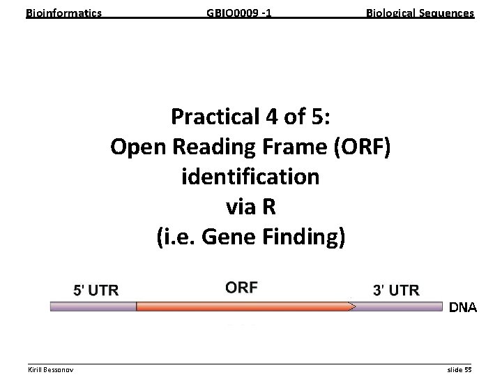
Bioinformatics GBIO 0009 1 Biological Sequences Practical 4 of 5: Open Reading Frame (ORF) identification via R (i. e. Gene Finding) __________________________________________________________ Kirill Bessonov slide 55

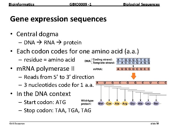
Bioinformatics GBIO 0009 1 Biological Sequences Gene expression sequences • Central dogma – DNA RNA protein • Each codon codes for one amino acid (a. a. ) – residue = amino acid • m. RNA polymerase II – Reads from 5’ to 3’ direction – 3 nucleotides code for 1 a. a. • In the DNA context – Start codon: ATG – Stop codon: TAA, TGA, TAG __________________________________________________________ Kirill Bessonov slide 56

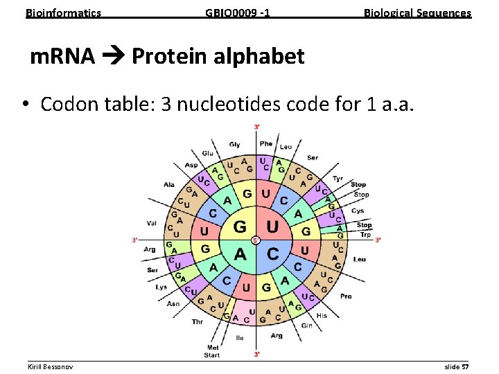
Bioinformatics GBIO 0009 1 Biological Sequences m. RNA Protein alphabet • Codon table: 3 nucleotides code for 1 a. a. __________________________________________________________ Kirill Bessonov slide 57

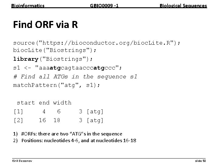
Bioinformatics GBIO 0009 1 Biological Sequences Find ORF via R source("https: //bioconductor. org/bioc. Lite. R"); bioc. Lite("Biostrings"); library("Biostrings"); s 1 <- "aaaatgcagtaacccatgccc"; # Find all ATGs in the sequence s 1 match. Pattern("atg", s 1); start end width [1] 4 6 [2] 16 18 3 [atg] 1) #ORFs: there are two “ATG”s in the sequence 2) Positions: nucleotides 4 6, and at nucleotides 16 18 __________________________________________________________ Kirill Bessonov slide 58

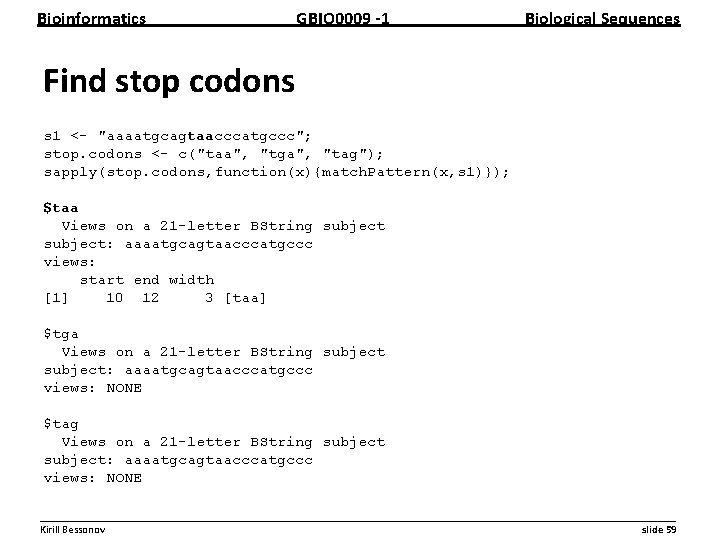
Bioinformatics GBIO 0009 1 Biological Sequences Find stop codons s 1 <- "aaaatgcagtaacccatgccc"; stop. codons <- c("taa", "tga", "tag"); sapply(stop. codons, function(x){match. Pattern(x, s 1)}); $taa Views on a 21 -letter BString subject: aaaatgcagtaacccatgccc views: start end width [1] 10 12 3 [taa] $tga Views on a 21 -letter BString subject: aaaatgcagtaacccatgccc views: NONE $tag Views on a 21 -letter BString subject: aaaatgcagtaacccatgccc views: NONE __________________________________________________________ Kirill Bessonov slide 59

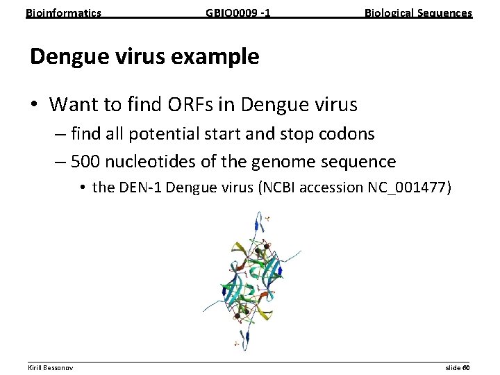
Bioinformatics GBIO 0009 1 Biological Sequences Dengue virus example • Want to find ORFs in Dengue virus – find all potential start and stop codons – 500 nucleotides of the genome sequence • the DEN 1 Dengue virus (NCBI accession NC_001477) __________________________________________________________ Kirill Bessonov slide 60

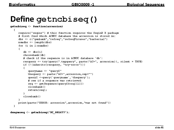
Bioinformatics GBIO 0009 1 Biological Sequences Define getncbiseq() getncbiseq <- function(accession) { require("seqinr") # this function requires the Seqin. R R package # first find which ACNUC database the accession is stored in: dbs <- c("genbank", "refseq. Viruses", "bacterial") numdbs <- length(dbs) for (i in 1: numdbs) { db <- dbs[i] choosebank(db) # check if the sequence is in ACNUC database 'db': resquery <- try(query(". tmpquery", paste("AC=", accession)), silent = TRUE) if (!(inherits(resquery, "try-error"))) { queryname <- "query 2" thequery <- paste("AC=", accession, sep="") query 2 <-query(`queryname`, `thequery`); # see if a sequence was retrieved: seq <- get. Sequence(query 2$req[[1]]) closebank() return(seq); } closebank() } print(paste("ERROR: accession", accession, "was not found")) } dengueseq <- getncbiseq("NC_001477"); __________________________________________________________ Kirill Bessonov slide 61

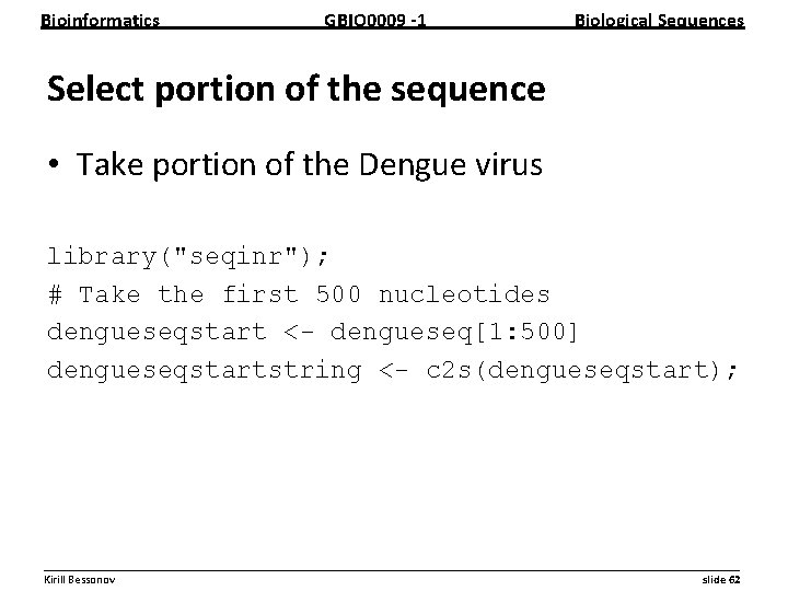
Bioinformatics GBIO 0009 1 Biological Sequences Select portion of the sequence • Take portion of the Dengue virus library("seqinr"); # Take the first 500 nucleotides dengueseqstart <- dengueseq[1: 500] dengueseqstartstring <- c 2 s(dengueseqstart); __________________________________________________________ Kirill Bessonov slide 62

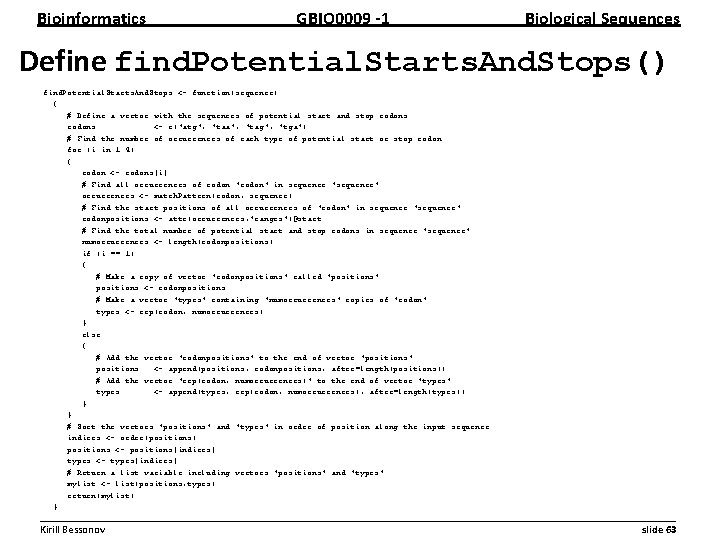
Bioinformatics GBIO 0009 1 Biological Sequences Define find. Potential. Starts. And. Stops() find. Potential. Starts. And. Stops <- function(sequence) { # Define a vector with the sequences of potential start and stop codons <- c("atg", "taa", "tag", "tga") # Find the number of occurrences of each type of potential start or stop codon for (i in 1: 4) { codon <- codons[i] # Find all occurrences of codon "codon" in sequence "sequence" occurrences <- match. Pattern(codon, sequence) # Find the start positions of all occurrences of "codon" in sequence "sequence" codonpositions <- attr(occurrences, "ranges")@start # Find the total number of potential start and stop codons in sequence "sequence" numoccurrences <- length(codonpositions) if (i == 1) { # Make a copy of vector "codonpositions" called "positions" positions <- codonpositions # Make a vector "types" containing "numoccurrences" copies of "codon" types <- rep(codon, numoccurrences) } else { # Add the vector "codonpositions" to the end of vector "positions": positions <- append(positions, codonpositions, after=length(positions)) # Add the vector "rep(codon, numoccurrences)" to the end of vector "types": types <- append(types, rep(codon, numoccurrences), after=length(types)) } } # Sort the vectors "positions" and "types" in order of position along the input sequence: indices <- order(positions) positions <- positions[indices] types <- types[indices] # Return a list variable including vectors "positions" and "types": mylist <- list(positions, types) return(mylist) } __________________________________________________________ Kirill Bessonov slide 63

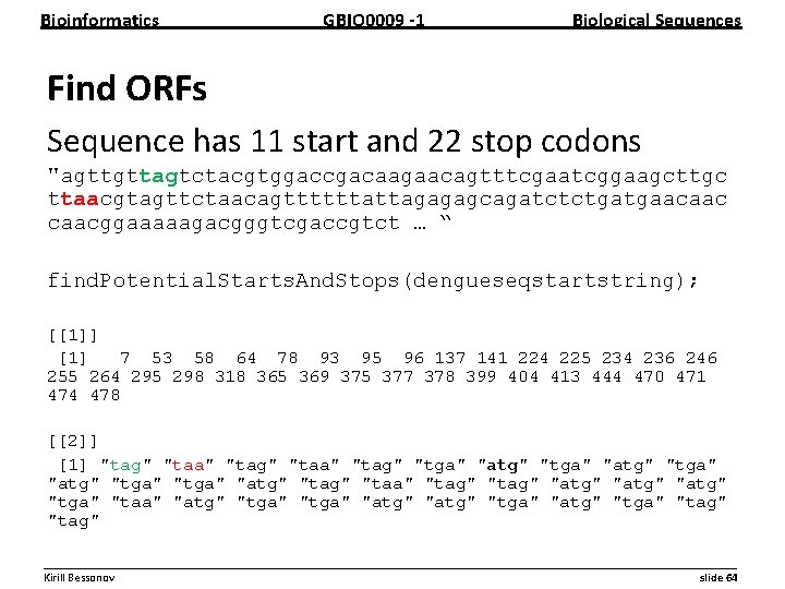
Bioinformatics GBIO 0009 1 Biological Sequences Find ORFs Sequence has 11 start and 22 stop codons "agttgttagtctacgtggaccgacaagaacagtttcgaatcggaagcttgc ttaacgtagttctaacagttttttattagagagcagatctctgatgaacaacggaaaaagacgggtcgaccgtct … “ find. Potential. Starts. And. Stops(dengueseqstartstring); [[1]] [1] 7 53 58 64 78 93 95 96 137 141 224 225 234 236 246 255 264 295 298 318 365 369 375 377 378 399 404 413 444 470 471 474 478 [[2]] [1] "tag" "taa" "tag" "tga" "atg" "tga" "atg" "taa" "tag" "atg" "tga" "taa" "atg" "tga" "atg" "tga" "tag" __________________________________________________________ Kirill Bessonov slide 64

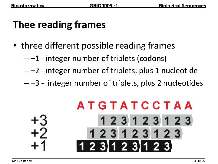
Bioinformatics GBIO 0009 1 Biological Sequences Thee reading frames • three different possible reading frames – +1 integer number of triplets (codons) – +2 integer number of triplets, plus 1 nucleotide – +3 integer number of triplets, plus 2 nucleotides __________________________________________________________ Kirill Bessonov slide 65

Bioinformatics GBIO 0009 1 Biological Sequences Identify reading frame • Get sub sequence substring(dengueseqstartstring, 137, 143); [1] "atgctga" • starts – a potential start codon (ATG) • ends – with a potential stop codon (TGA) • there is – an integer number of triplets – plus one nucleotide – frame +2 __________________________________________________________ Kirill Bessonov slide 66

Bioinformatics GBIO 0009 1 Biological Sequences Find ORF in DNA • Search for – a potential start codon, – followed by an integer number of codons, – followed by a potential stop codon – test all 3 frames • Input 500 bp of the DEN 1 virus __________________________________________________________ Kirill Bessonov slide 67

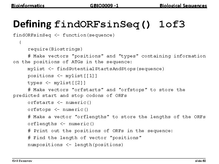
Bioinformatics GBIO 0009 1 Biological Sequences Defining find. ORFsin. Seq() 1 of 3 find. ORFsin. Seq <- function(sequence) { require(Biostrings) # Make vectors "positions" and "types" containing information on the positions of ATGs in the sequence: mylist <- find. Potential. Starts. And. Stops(sequence) positions <- mylist[[1]] types <- mylist[[2]] # Make vectors "orfstarts" and "orfstops" to store the predicted start and stop codons of ORFs orfstarts <- numeric() orfstops <- numeric() # Make a vector "orflengths" to store the lengths of the ORFs orflengths <- numeric() # Print out the positions of ORFs in the sequence: # Find the length of vector "positions" numpositions <- length(positions) __________________________________________________________ Kirill Bessonov slide 68

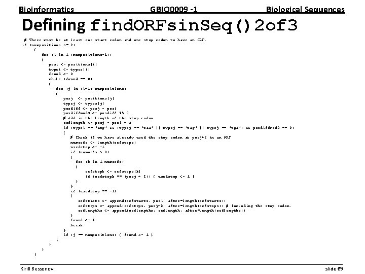
Bioinformatics GBIO 0009 1 Biological Sequences Defining find. ORFsin. Seq()2 of 3 # There must be at least one start codon and one stop codon to have an ORF. if (numpositions >= 2) { for (i in 1: (numpositions-1)) { posi <- positions[i] typei <- types[i] found <- 0 while (found == 0) { for (j in (i+1): numpositions) { posj <- positions[j] typej <- types[j] posdiff <- posj - posi posdiffmod 3 <- posdiff %% 3 # Add in the length of the stop codon orflength <- posj - posi + 3 if (typei == "atg" && (typej == "taa" || typej == "tag" || typej == "tga") && posdiffmod 3 == 0) { # Check if we have already used the stop codon at posj+2 in an ORF numorfs <- length(orfstops) usedstop <- -1 if (numorfs > 0) { for (k in 1: numorfs) { orfstopk <- orfstops[k] if (orfstopk == (posj + 2)) { usedstop <- 1 } } } if (usedstop == -1) { orfstarts <- append(orfstarts, posi, after=length(orfstarts)) orfstops <- append(orfstops, posj+2, after=length(orfstops)) # Including the stop codon. orflengths <- append(orflengths, orflength, after=length(orflengths)) } found <- 1 break } if (j == numpositions) { found <- 1 } } } __________________________________________________________ Kirill Bessonov slide 69

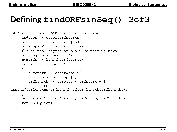
Bioinformatics GBIO 0009 1 Biological Sequences Defining find. ORFsin. Seq() 3 of 3 # Sort the final ORFs by start position: indices <- order(orfstarts) orfstarts <- orfstarts[indices] orfstops <- orfstops[indices] # Find the lengths of the ORFs that we have orflengths <- numeric() numorfs <- length(orfstarts) for (i in 1: numorfs) { orfstart <- orfstarts[i] orfstop <- orfstops[i] orflength <- orfstop - orfstart + 1 orflengths <append(orflengths, orflength, after=length(orflengths)) } mylist <- list(orfstarts, orfstops, orflengths) return(mylist) } __________________________________________________________ Kirill Bessonov slide 70

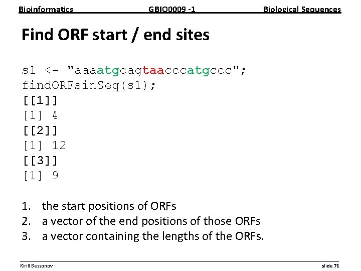
Bioinformatics GBIO 0009 1 Biological Sequences Find ORF start / end sites s 1 <- "aaaatgcagtaacccatgccc"; find. ORFsin. Seq(s 1); [[1]] [1] 4 [[2]] [1] 12 [[3]] [1] 9 1. the start positions of ORFs 2. a vector of the end positions of those ORFs 3. a vector containing the lengths of the ORFs. __________________________________________________________ Kirill Bessonov slide 71

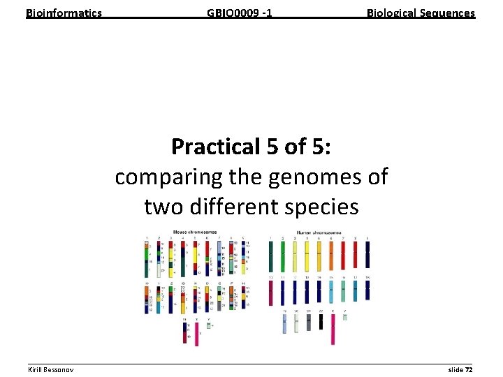
Bioinformatics GBIO 0009 1 Biological Sequences Practical 5 of 5: comparing the genomes of two different species __________________________________________________________ Kirill Bessonov slide 72

Bioinformatics GBIO 0009 1 Biological Sequences Comparison • Comparative genomics – Compares genomes • two different species, or • two different strains • Do the two species have the same number of genes? • Which genes were gained or lost? __________________________________________________________ Kirill Bessonov slide 73

Bioinformatics GBIO 0009 1 Biological Sequences Tuning bioma. Rt # Load the bioma. Rt package in R library("bioma. Rt"); # List all databases that can be queried list. Marts(); 1. The names of the databases are listed and version 2. Can query many different databases including Worm. Base, Uni. Prot, Ensembl, etc. __________________________________________________________ Kirill Bessonov slide 74

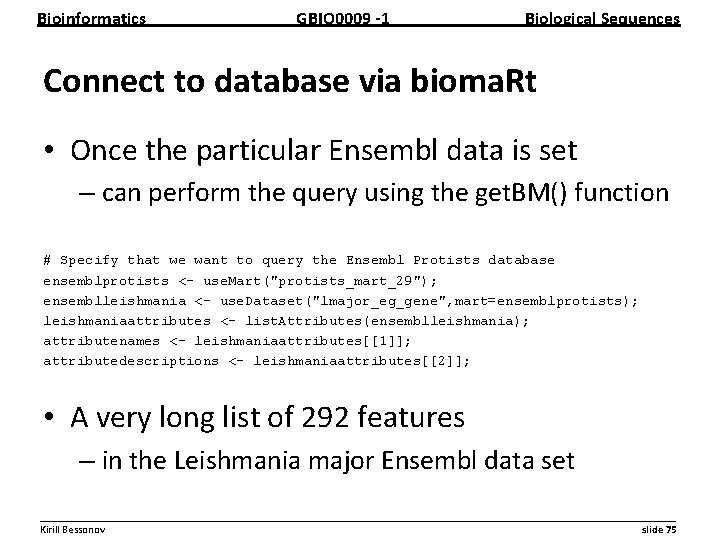
Bioinformatics GBIO 0009 1 Biological Sequences Connect to database via bioma. Rt • Once the particular Ensembl data is set – can perform the query using the get. BM() function # Specify that we want to query the Ensembl Protists database ensemblprotists <- use. Mart("protists_mart_29"); ensemblleishmania <- use. Dataset("lmajor_eg_gene", mart=ensemblprotists); leishmaniaattributes <- list. Attributes(ensemblleishmania); attributenames <- leishmaniaattributes[[1]]; attributedescriptions <- leishmaniaattributes[[2]]; • A very long list of 292 features – in the Leishmania major Ensembl data set __________________________________________________________ Kirill Bessonov slide 75

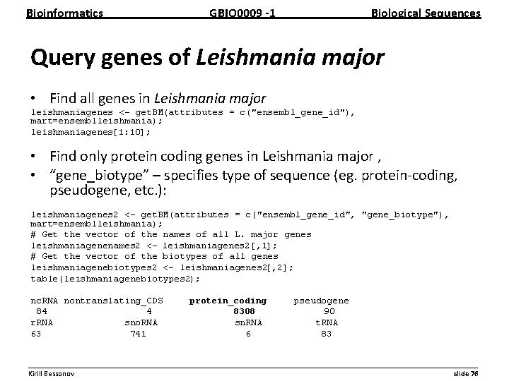
Bioinformatics GBIO 0009 1 Biological Sequences Query genes of Leishmania major • Find all genes in Leishmania major leishmaniagenes <- get. BM(attributes = c("ensembl_gene_id"), mart=ensemblleishmania); leishmaniagenes[1: 10]; • Find only protein coding genes in Leishmania major , • “gene_biotype” – specifies type of sequence (eg. protein coding, pseudogene, etc. ): leishmaniagenes 2 <- get. BM(attributes = c("ensembl_gene_id", "gene_biotype"), mart=ensemblleishmania); # Get the vector of the names of all L. major genes leishmaniagenenames 2 <- leishmaniagenes 2[, 1]; # Get the vector of the biotypes of all genes leishmaniagenebiotypes 2 <- leishmaniagenes 2[, 2]; table(leishmaniagenebiotypes 2); nc. RNA nontranslating_CDS 84 4 r. RNA sno. RNA 63 741 protein_coding 8308 sn. RNA 6 pseudogene 90 t. RNA 83 __________________________________________________________ Kirill Bessonov slide 76

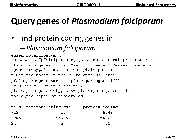
Bioinformatics GBIO 0009 1 Biological Sequences Query genes of Plasmodium falciparum • Find protein coding genes in – Plasmodium falciparum ensemblpfalciparum <use. Dataset("pfalciparum_eg_gene", mart=ensemblprotists); pfalciparumgenes <- get. BM(attributes = c("ensembl_gene_id", "gene_biotype"), mart=ensemblpfalciparum); # Get the names of the P. falciparum genes pfalciparumgenenames <- pfalciparumgenes[[1]]; length(pfalciparumgenenames); pfalciparumgenebiotypes <- pfalciparumgenes[[2]]; table(pfalciparumgenebiotypes); nc. RNA nontranslating_cds 712 80 r. RNA sn. RNA 24 3 protein_coding 5349 t. RNA 45 __________________________________________________________ Kirill Bessonov slide 77

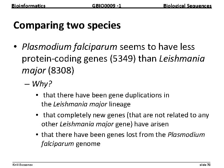
Bioinformatics GBIO 0009 1 Biological Sequences Comparing two species • Plasmodium falciparum seems to have less protein coding genes (5349) than Leishmania major (8308) – Why? • that there have been gene duplications in the Leishmania major lineage • that completely new genes (that are not related to any other Leishmania major gene) have arisen • that there have been genes lost from the Plasmodium falciparum genome __________________________________________________________ Kirill Bessonov slide 78

Bioinformatics GBIO 0009 1 Biological Sequences __________________________________________________________ Kirill Bessonov slide 79

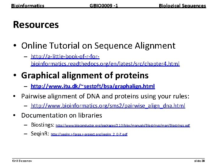
Bioinformatics GBIO 0009 1 Biological Sequences Resources • Online Tutorial on Sequence Alignment – http: //a little book of r for bioinformatics. readthedocs. org/en/latest/src/chapter 4. html • Graphical alignment of proteins – http: //www. itu. dk/~sestoft/bsa/graphalign. html • Pairwise alignment of DNA and proteins using your rules: – http: //www. bioinformatics. org/sms 2/pairwise_align_dna. html • Documentation on libraries – Biostings: http: //www. bioconductor. org/packages/2. 10/bioc/manuals/Biostrings/man/Biostrings. pdf – Seqin. R: http: //seqinr. r forge. r project. org/seqinr_2_0 7. pdf __________________________________________________________ Kirill Bessonov slide 80