Bioinformatics Algorithms and Data Structures CLUSTAL W Algorithm

Bioinformatics Algorithms and Data Structures CLUSTAL W Algorithm Lecturer: Dr. Rose Slides by: Dr. Rose March 29, 2007 UNIVERSITY OF SOUTH CAROLINA College of Engineering & Information Technology

Multiple Sequence Alignment • CLUSTAL is an algorithm for aligning multiple sequences. • Reasons for computing multiple alignments: – Characterizing protein families – Detect homology between sequences and families of sequences – Predict secondary and tertiary structures of new sequences. – Needed for creating of phylogenetic trees. UNIVERSITY OF SOUTH CAROLINA College of Engineering & Information Technology

Multiple Sequence Alignment • Recall: DP used for 2 sequence alignment – Guarantees optimal alignment relative to the scoring table that is used. – DP is only practical for small numbers of short sequences. – Impractical for: • large numbers of sequences • Very long sequences • i. e. , more than 8 proteins of average length. UNIVERSITY OF SOUTH CAROLINA College of Engineering & Information Technology

Progressive Algorithms • Progressive Approaches – Exploit idea that homologous sequences are related by evolution. – Multiple alignments can be built up from pairwise alignments. – The pairwise alignments follow branching in the guide tree. Q: What is a guide tree? – The most closely related sequences are aligned first. – The more distant related sequences are gradually added. UNIVERSITY OF SOUTH CAROLINA College of Engineering & Information Technology

Progressive Algorithms • Empirical observations: – For simple cases: • correctly align domains of known secondary and tertiary structures. • closely related sequences are less sensitive to parameter settings, i. e. , gap penalties and weight matrix. – In all cases: • gaps are preserved, i. e. , once a gap always a gap. • progressive alignment gives an idea of the variability at each position before more distant sequences are added. UNIVERSITY OF SOUTH CAROLINA College of Engineering & Information Technology

Progressive Algorithms • Empirical observations: – For more complicated cases: • Progressive approach is less reliable for highly divergent sequences (less than 25 -30% identity). • gives a good starting point for further manual/automatic refinement. UNIVERSITY OF SOUTH CAROLINA College of Engineering & Information Technology

Problems with Progressive Algorithms • Local minimum problem – Recall this is a greedy algorithm approach – Sequences are added greedily: • Multiple alignments are built up from pairwise alignments. • The pairwise alignments follow branching in the initial guide tree. (more on this later) – No guarantee of a global optimum – Any misaligned regions made early on can not be corrected later on. UNIVERSITY OF SOUTH CAROLINA College of Engineering & Information Technology

Problems with Progressive Algorithms • Sensitivity to alignment parameters – problematic also for iterative and stochastic algorithms. – Traditional parameters: • weight table • cost of opening a gap • cost of extending a gap – Expectation is one set of parameters works well over • all sequences in the set • all parts of each sequence UNIVERSITY OF SOUTH CAROLINA College of Engineering & Information Technology

Problems with Progressive Algorithms • Sensitivity to alignment parameters continued – A single weight matrix choice will generally work for closely related sequences. • weight matrices give highest weight to identities • Any weight matrix will work ok if identities dominate – For divergent sequences: • Nonidentical residues are more significant • Scores to these residues are critical • Different weight matrices will be required for: – different evolutionary distances – Different classes of proteins UNIVERSITY OF SOUTH CAROLINA College of Engineering & Information Technology

Problems with Progressive Algorithms • Sensitivity to alignment parameters continued – A range of gap penalty values will generally work for closely related sequences. – For divergent sequences: • The specific choice of gap penalty value becomes critical • For proteins gaps don’t occur randomly. – Recall our discussion of conserved secondary features – Gaps occur between alpha helices and beta strands rather than within them UNIVERSITY OF SOUTH CAROLINA College of Engineering & Information Technology

CLUSTAL W Contributions • Dynamically vary gap penalties according to position & residue • Local gap opening penalty adjustment: – relative to observed relative frequency of gaps next to each of the 20 amino acid. – reduced for loop or random coil regions (as indicated by short stretches of hydrophilic residues) – reduced for gaps found in early alignments – increased within 8 residues of existing gaps (observation: gaps tend not to be closer than 8 residues) UNIVERSITY OF SOUTH CAROLINA College of Engineering & Information Technology

CLUSTAL W Contributions • Weight matrices are chosen dynamically – PAM series and BLOSUM series are main series of amino acid weight matrices in use. – Choice of weight matrix is by estimation of divergence of sequences being aligned at each step. – Different weight matrices are appropriate depending on similarity of sequences UNIVERSITY OF SOUTH CAROLINA College of Engineering & Information Technology

CLUSTAL W Contributions – Different weight matrices are appropriate depending on similarity of sequences: • For closely related sequences: – identities predominate – Only frequent conservative substitutions are scored high • For evolutionary divergent sequences: – Less weight should be given to identities – Weight matrix should be tuned to greater evolutionary distance UNIVERSITY OF SOUTH CAROLINA College of Engineering & Information Technology

CLUSTAL W Contributions • Weighting of sequences: – corrects for unequal sampling across the evolutionary distance in the data set. • Downweights similar sequences • Upweights divergent sequences • Weight are calculated from the branch lengths of the initial guide tree. UNIVERSITY OF SOUTH CAROLINA College of Engineering & Information Technology

CLUSTAL W Contributions • Neighbor-Joining method used to calculate guide tree – Less sensitive to unequal evolutionary rates in different branches. – Significance: branch lengths are used to derive sequence weights. – Accuracy of distance calculations for guide tree: • Tree constructed from pairwise distance matrix • User selectable: – Fast approximate alignment – Full dynamic programming UNIVERSITY OF SOUTH CAROLINA College of Engineering & Information Technology

CLUSTAL W Algorithm Basic method: 1. Distance matrix is calculated • • Distances are pairwise alignment scores Gives divergence of each pair of sequences 2. Guide tree built from distance matrix 3. Progressive alignment according to guide tree • • Branching order of tree specifies alignment order Alignment progresses from leaves to root. UNIVERSITY OF SOUTH CAROLINA College of Engineering & Information Technology

CLUSTAL W Algorithm Distance matrix/pairwise alignments phase – Two choices: fast approximation or DP – Fast approximation: • Defn a k-tuple match is a run of identical residues, typically – 1 to 2 for proteins – 2 to 4 for nucleotide sequences • Scores are calculated as: (k-tuple matches) – fixed penalty per gap • Score is initially calculated as a percent identity score. • Distance = 1. 0 – (score/100) UNIVERSITY OF SOUTH CAROLINA College of Engineering & Information Technology

CLUSTAL W Algorithm Distance matrix/pairwise alignments phase – Full DP alignment • Alignment uses: 1. gap opening penalties 2. gap extension penalties 3. full amino acid weight matrix. • • • Scores are calculated as: (#identies)/(#residues), gaps not included Score is initially calculated as a percent identity score. Distance = 1. 0 – (score/100) UNIVERSITY OF SOUTH CAROLINA College of Engineering & Information Technology

NJ Algorithm Neighbor Joining to Calculate the Guide Tree Phase: – – does not require a uniform molecular clock the raw data are provided as a distance matrix the initial tree is a star tree distance matrix is modified • distance between node pairs is adjusted on the basis of their average divergence from all other nodes. – the least-distant pair of nodes are linked. UNIVERSITY OF SOUTH CAROLINA College of Engineering & Information Technology

NJ Algorithm Neighbor Joining to Calculate the Guide Tree Phase: – When two nodes are linked: • Add their common ancestral node to the tree • delete the terminal nodes with their branches • the common ancestor is now a terminal node on a smaller tree – At each step, two terminal nodes are replaced by one new node – The process is complete when there are only two nodes separated by a single branch UNIVERSITY OF SOUTH CAROLINA College of Engineering & Information Technology

NJ Algorithm • Advantages of Neighbor Joining – Fast. • Can be used on large datasets • Can support bootstrap analysis – Can handle lineages with largely different branch lengths (different molecular evolutionary rates) – Can be used with methods that use correction for multiple substitutions UNIVERSITY OF SOUTH CAROLINA College of Engineering & Information Technology

NJ Algorithm • Disadvantages of Neighbor Joining – sequence information is reduced • Sequences are boiled down to distances • No secondary or tertiary features used – gives only one possible tree – strongly dependent on the model of evolution used UNIVERSITY OF SOUTH CAROLINA College of Engineering & Information Technology

NJ Algorithm • NJ example from: http: //www. icp. ucl. ac. be/~opperd/private/neighbor. html • Consider the following tree: • Notice that the branches for D and B are longer. • This expresses the idea that they have a faster molecular clock than the other OTUs. UNIVERSITY OF SOUTH CAROLINA College of Engineering & Information Technology

NJ Algorithm The distance matrix for the tree is: Normally, we create the tree from the distances. In this example, we use to tree to derive the distances. UNIVERSITY OF SOUTH CAROLINA College of Engineering & Information Technology

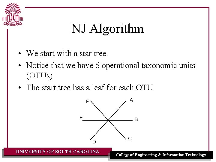
NJ Algorithm • We start with a star tree. • Notice that we have 6 operational taxonomic units (OTUs) • The start tree has a leaf for each OTU UNIVERSITY OF SOUTH CAROLINA College of Engineering & Information Technology

NJ Algorithm Step 1: Calculate the net divergence for each OTU. The net divergence is the sum of distances from i to all other OTUs. r(A) = 5+4+7+6+8=30 r(B) = 42 r(C) = 32 r(D) = 38 r(E) = 34 r(F) = 44 UNIVERSITY OF SOUTH CAROLINA College of Engineering & Information Technology

NJ Algorithm Step 2: Calculate a new distance matrix based on average divergence: M(ij)=d(ij) - [r(i) + r(j)]/(N-2) Example: A, B M(AB)=d(AB) -[(r(A) + r(B)]/(N-2) = -13 Recall: r(A) =30 r(B) = 42 UNIVERSITY OF SOUTH CAROLINA College of Engineering & Information Technology

NJ Algorithm Step 2: continued M(ij)=d(ij) - [r(i) + r(j)]/(N-2) Distance matrix UNIVERSITY OF SOUTH CAROLINA Average divergence matrix College of Engineering & Information Technology

NJ Algorithm Step 3: choose two OTUs for which Mij is the smallest. – – the possible choices are: A, B and D, E arbitrarily choose A and B form a new node called U, the parent of A & B. calculate the branch length from U to A and B. S(AU) =d(AB) / 2 + [r(A)-r(B)] / 2(N-2) = 1 S(BU) =d(AB) -S(AU) = 4 UNIVERSITY OF SOUTH CAROLINA College of Engineering & Information Technology

NJ Algorithm • The tree after U is added. UNIVERSITY OF SOUTH CAROLINA College of Engineering & Information Technology

NJ Algorithm Step 4: define distances from U to other terminal nodes: – – – d(CU) = d(AC) + d(BC) - d(AB) / 2 = 3 d(DU) = d(AD) + d(BD) - d(AB) / 2 = 6 d(EU) = d(AE) + d(BE) - d(AB) / 2 = 5 d(FU) = d(AF) + d(BF) - d(AB) / 2 = 7 Note: no change in paired distances {C, D, E, F} UNIVERSITY OF SOUTH CAROLINA College of Engineering & Information Technology

NJ Algorithm • Now N = N-1 = 5 • Repeat steps 1 through 4 • Stop when N = 2 UNIVERSITY OF SOUTH CAROLINA College of Engineering & Information Technology

CLUSTAL W Algorithm • The final result of the tree produced by NJ is an unrooted tree. • The branch lengths are proportional to the estimated divergence. • A “mid-point” method is used to place the root: – The mid point is defined at the point where the means of the branch lengths on either side are equal. UNIVERSITY OF SOUTH CAROLINA College of Engineering & Information Technology

CLUSTAL W Algorithm Basic Progressive Alignment Phase: – Use a series of pairwise alignments – The alignments follow the branching order of the guide tree – The alignments start from the leaves and progress towards the root – Full DP with a residue weight matrix is used – Gaps are preserved – Newly created gaps get full opening & extension penalties UNIVERSITY OF SOUTH CAROLINA College of Engineering & Information Technology

CLUSTAL W Algorithm Basic Progressive Alignment Phase: – Each step involved two existing alignments or sequences – The score at a given position is the average of the pairwise weight matrix scores. Example: • aligning 2 alignments: with 3 and 4 sequences, respectively • The score at a given position is the average of the 3 X 4 comparisons. • The weight matrix has only positive scores • Each gap versus a residue is scored a zero, the worst value • This is the average linkage cluster distance metric UNIVERSITY OF SOUTH CAROLINA College of Engineering & Information Technology

CLUSTAL W Algorithm Example: 1. 2. 3. 4. 5. A & B are aligned C is aligned with the result of (1) D & E are aligned The results of (2) and (3) are aligned F is aligned with the result of (4) UNIVERSITY OF SOUTH CAROLINA College of Engineering & Information Technology

CLUSTAL W Algorithm Improvement to Progressive Alignment Phase: – Sequence weighting: • Calculated from the guide tree • Normalized so that largest weight is 1. 0 • Closely related sequences receive lower weights – They over-represent their common information – A lower weight seeks to reduce this influence • Divergent sequences receive higher weights • Sequence weight impacts alignment scores: – each weight matrix value is multiplied by the weights of the two sequences. UNIVERSITY OF SOUTH CAROLINA College of Engineering & Information Technology

CLUSTAL W Algorithm Improvement to Progressive Alignment Phase: – Two gap penalty types: • Gap opening (GOP) • Gap extension (GEP) – Actual assessed penalty depends on: • Weight matrix: GOP is scaled by the average score of mismatched residues • Similarity of sequences: % identity is used to » increase GOP for similar sequences » decrease GOP for divergent sequences UNIVERSITY OF SOUTH CAROLINA College of Engineering & Information Technology

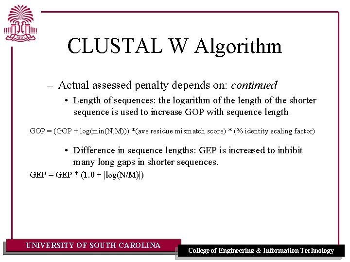
CLUSTAL W Algorithm – Actual assessed penalty depends on: continued • Length of sequences: the logarithm of the length of the shorter sequence is used to increase GOP with sequence length GOP = (GOP + log(min(N, M))) *(ave residue mismatch score) * (% identity scaling factor) • Difference in sequence lengths: GEP is increased to inhibit many long gaps in shorter sequences. GEP = GEP * (1. 0 + |log(N/M)|) UNIVERSITY OF SOUTH CAROLINA College of Engineering & Information Technology

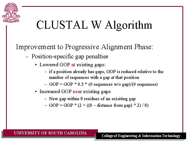
CLUSTAL W Algorithm Improvement to Progressive Alignment Phase: – Position-specific gap penalties • Lowered GOP at existing gaps: – if a position already has gaps, GOP is reduced relative to the number of sequences with a gap at that position – GOP = GOP * 0. 3 * (# sequences w/o gap)/(# sequences) • Increased GOP near existing gaps – New gap within 8 residues of an exisiting gap – GOP = GOP * (2 + ((8 – distance from gap) * 2) / 8) UNIVERSITY OF SOUTH CAROLINA College of Engineering & Information Technology

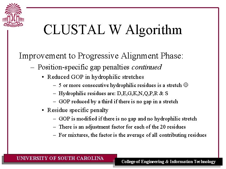
CLUSTAL W Algorithm Improvement to Progressive Alignment Phase: – Position-specific gap penalties continued • Reduced GOP in hydrophilic stretches – 5 or more consecutive hydrophilic residues is a stretch – Hydrophilic residues are: D, E, G, K, N, Q, P, R & S – GOP reduced by a third if there is no gap in a stretch • Residue specific penalty – GOP is modified if there is no gap and no hydrophilic stretch – There is an adjustment factor for each of the 20 residues – For mixtures, the factor is the average of all contributing residues UNIVERSITY OF SOUTH CAROLINA College of Engineering & Information Technology

The End UNIVERSITY OF SOUTH CAROLINA College of Engineering & Information Technology