Bioinformatics 3 V 9 Dynamic Regulation Petri Boolean

Bioinformatics 3 V 9 – Dynamic Regulation: Petri & Boolean Networks Mon, Nov 12, 2011

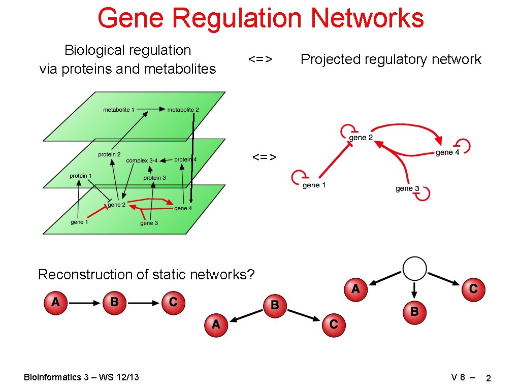
Gene Regulation Networks Biological regulation via proteins and metabolites <=> Projected regulatory network <=> Reconstruction of static networks? Bioinformatics 3 – WS 12/13 V 8 – 2

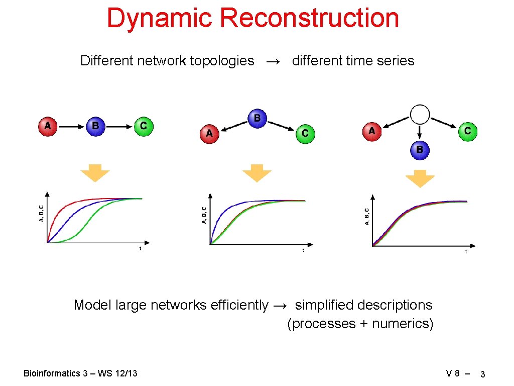
Dynamic Reconstruction Different network topologies → different time series Model large networks efficiently → simplified descriptions (processes + numerics) Bioinformatics 3 – WS 12/13 V 8 – 3

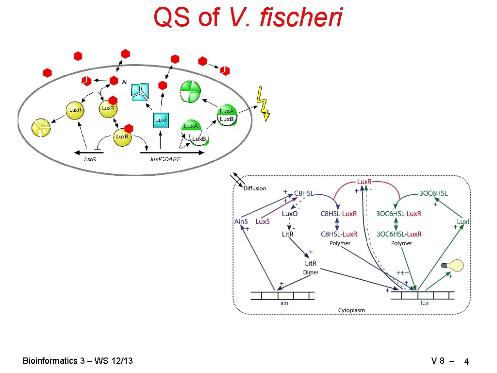
QS of V. fischeri Bioinformatics 3 – WS 12/13 V 8 – 4

Boolean Networks "Blackboard explanations" often formulated as conditional transitions • "If Lux. I is present, then AI will be produced…" • "If there is AI and there's no Lux. R: AI bound to the genome, then Lux. R will be expressed and complexes can form…" • "If Lux. R: AI is bound to the genome, then Lux. I is expressed…" Simplified mathematical description of the dependencies: Densities of the species <=> discrete states: on/off, 1/0 Network of dependencies <=> condition tables Progress in time <=> discrete propagation steps Bioinformatics 3 – WS 12/13 V 8 – 5

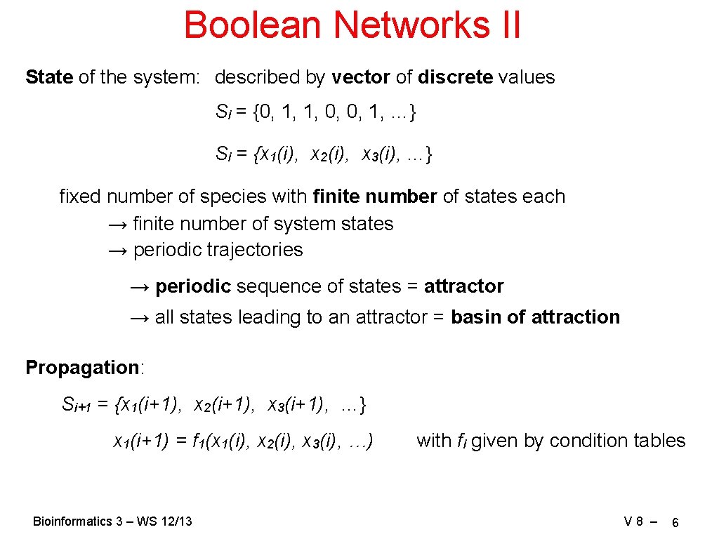
Boolean Networks II State of the system: described by vector of discrete values Si = {0, 1, 1, 0, 0, 1, …} Si = {x 1(i), x 2(i), x 3(i), …} fixed number of species with finite number of states each → finite number of system states → periodic trajectories → periodic sequence of states = attractor → all states leading to an attractor = basin of attraction Propagation: Si+1 = {x 1(i+1), x 2(i+1), x 3(i+1), …} x 1(i+1) = f 1(x 1(i), x 2(i), x 3(i), …) Bioinformatics 3 – WS 12/13 with fi given by condition tables V 8 – 6

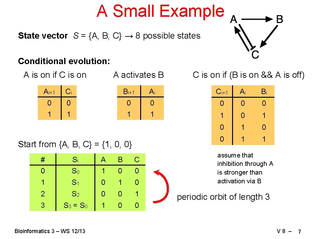
A Small Example State vector S = {A, B, C} → 8 possible states Conditional evolution: A is on if C is on A activates B C is on if (B is on && A is off) Ai+1 Ci Bi+1 Ai Ci+1 Ai Bi 0 0 0 0 1 1 1 0 1 0 0 1 1 Start from {A, B, C} = {1, 0, 0} # Si A B C 0 S 0 1 0 0 1 S 1 0 2 S 2 0 0 1 3 S 3 = S 0 1 0 0 Bioinformatics 3 – WS 12/13 assume that inhibition through A is stronger than activation via B periodic orbit of length 3 V 8 – 7

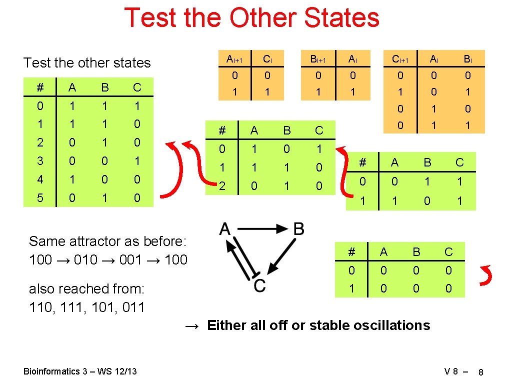
Test the Other States Test the other states # A B C 0 1 1 1 0 2 0 1 0 3 0 0 1 4 1 0 0 5 0 1 0 Same attractor as before: 100 → 010 → 001 → 100 also reached from: 110, 111, 101, 011 Ai+1 Ci Bi+1 Ai Ci+1 Ai Bi 0 0 0 0 1 1 1 0 1 0 0 1 1 # A B C 0 1 1 1 1 0 # A B C 2 0 1 0 0 0 1 1 0 1 # A B C 0 0 1 0 0 0 → Either all off or stable oscillations Bioinformatics 3 – WS 12/13 V 8 – 8

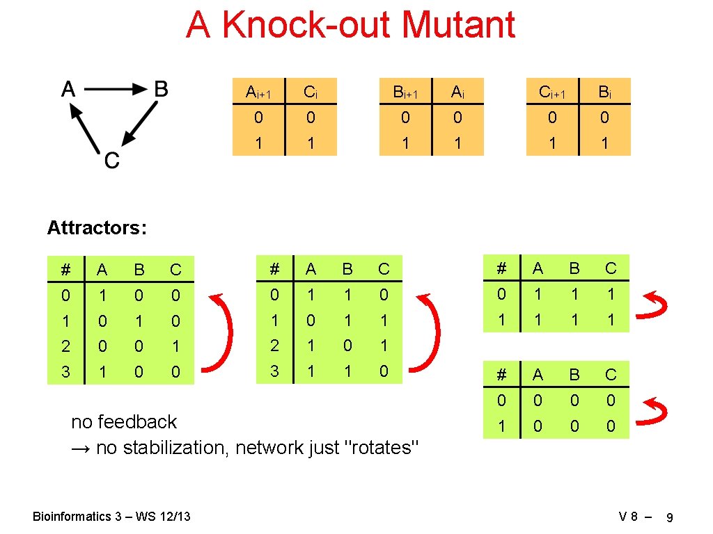
A Knock-out Mutant Ai+1 Ci Bi+1 Ai Ci+1 Bi 0 0 0 1 1 1 Attractors: # A B C 0 1 0 0 0 1 1 1 1 0 1 0 1 1 1 2 0 0 1 2 1 0 1 3 1 0 0 3 1 1 0 # A B C 0 0 1 0 0 0 no feedback → no stabilization, network just "rotates" Bioinformatics 3 – WS 12/13 V 8 – 9

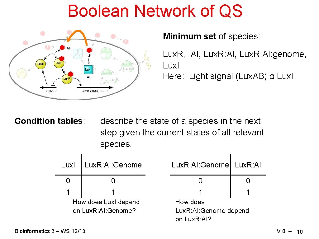
Boolean Network of QS Minimum set of species: Lux. R, AI, Lux. R: AI: genome, Lux. I Here: Light signal (Lux. AB) α Lux. I Condition tables: describe the state of a species in the next step given the current states of all relevant species. Lux. I Lux. R: AI: Genome 0 0 1 1 How does Lux. I depend on Lux. R: AI: Genome? Bioinformatics 3 – WS 12/13 Lux. R: AI: Genome Lux. R: AI How does Lux. R: AI: Genome depend on Lux. R: AI? V 8 – 10

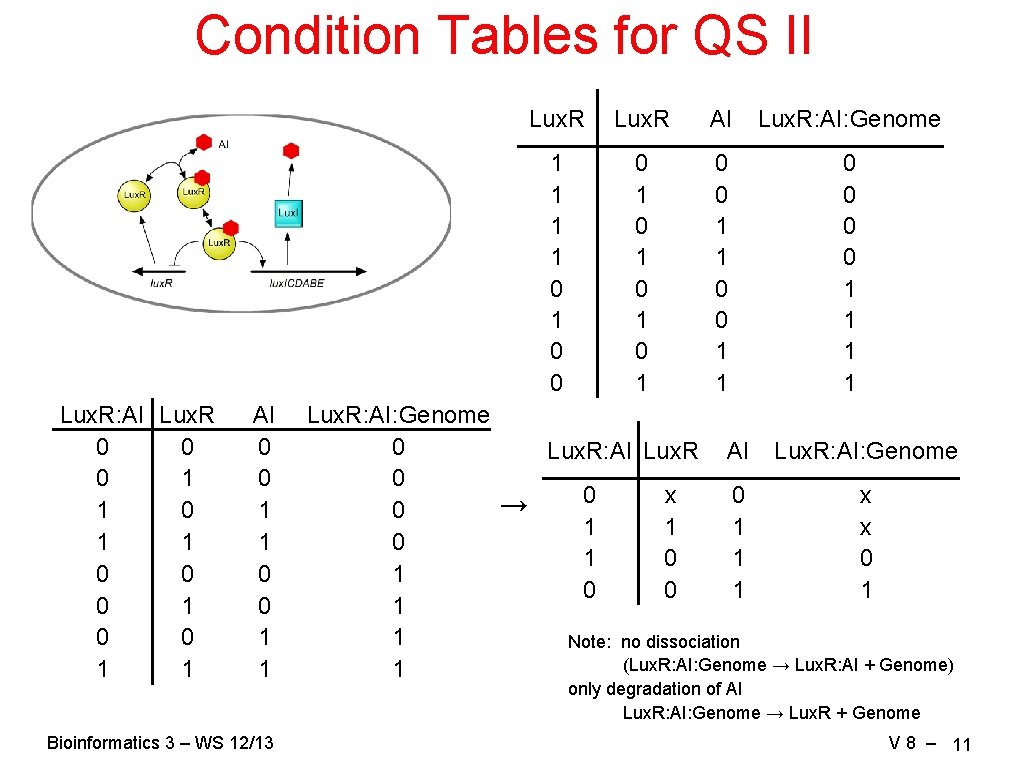
Condition Tables for QS II Lux. R: AI Lux. R 0 0 0 1 1 AI 0 0 1 1 Bioinformatics 3 – WS 12/13 Lux. R AI Lux. R: AI: Genome 1 1 0 1 0 0 0 1 0 1 0 0 1 1 Lux. R: AI: Genome 0 Lux. R: AI: Genome 0 0 x → 0 1 1 1 x 0 1 0 1 0 0 1 1 Note: no dissociation (Lux. R: AI: Genome → Lux. R: AI + Genome) 1 only degradation of AI Lux. R: AI: Genome → Lux. R + Genome V 8 – 11

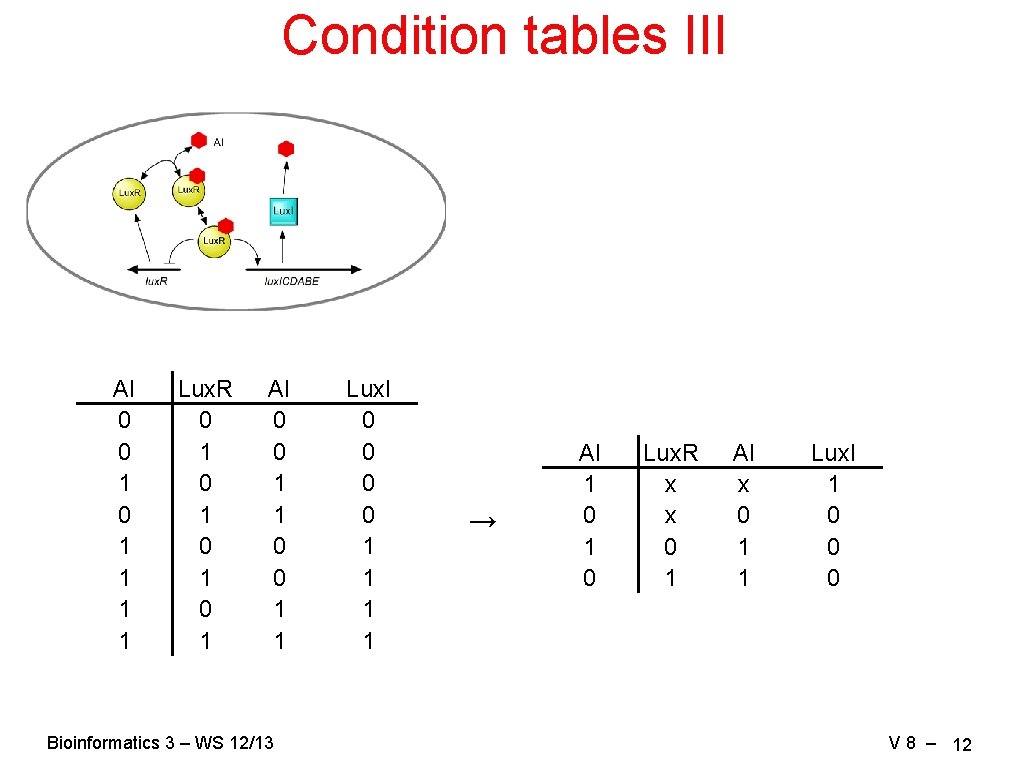
Condition tables III AI 0 0 1 1 1 1 Lux. R 0 1 0 1 AI 0 0 1 1 Bioinformatics 3 – WS 12/13 Lux. I 0 0 1 1 → AI 1 0 Lux. R x x 0 1 AI x 0 1 1 Lux. I 1 0 0 0 V 8 – 12

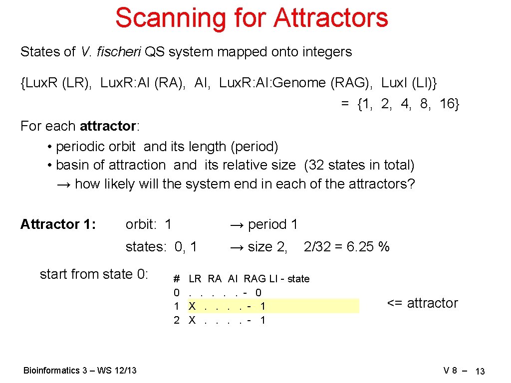
Scanning for Attractors States of V. fischeri QS system mapped onto integers {Lux. R (LR), Lux. R: AI (RA), AI, Lux. R: AI: Genome (RAG), Lux. I (LI)} = {1, 2, 4, 8, 16} For each attractor: • periodic orbit and its length (period) • basin of attraction and its relative size (32 states in total) → how likely will the system end in each of the attractors? Attractor 1: orbit: 1 → period 1 states: 0, 1 → size 2, start from state 0: Bioinformatics 3 – WS 12/13 # 0 1 2 2/32 = 6. 25 % LR RA AI RAG LI - state. . . - 0 X. . . . - 1 <= attractor V 8 – 13

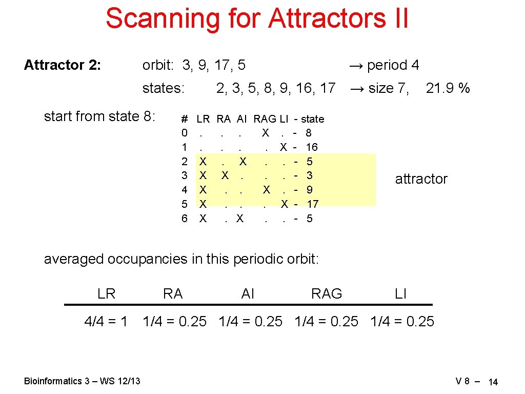
Scanning for Attractors II Attractor 2: orbit: 3, 9, 17, 5 states: start from state 8: → period 4 2, 3, 5, 8, 9, 16, 17 → size 7, # LR RA AI RAG LI - state 0. . . X. - 8 1. . X - 16 2 X. X. . - 5 3 X X. . . - 3 4 X. - 9 5 X. . . X - 17 6 X. X. . - 5 21. 9 % attractor averaged occupancies in this periodic orbit: LR RA AI RAG LI 4/4 = 1 1/4 = 0. 25 Bioinformatics 3 – WS 12/13 V 8 – 14

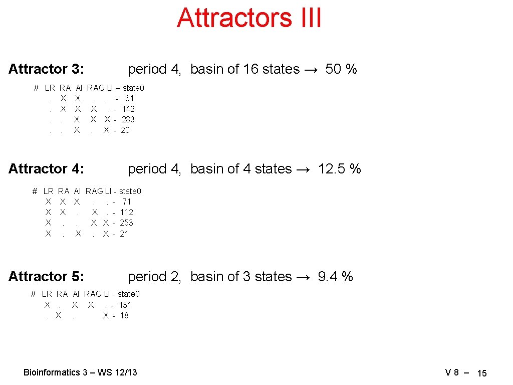
Attractors III Attractor 3: # LR. . RA X X. . period 4, basin of 16 states → 50 % AI RAG LI – state 0 X. . - 61 X X. - 142 X X X - 283 X. X - 20 Attractor 4: period 4, basin of 4 states → 12. 5 % # LR RA AI RAG LI - state 0 X X X. . - 71 X X. X. - 112 X. . X X - 253 X. X. X - 21 Attractor 5: period 2, basin of 3 states → 9. 4 % # LR RA AI RAG LI - state 0 X. X X. - 131. X. X - 18 Bioinformatics 3 – WS 12/13 V 8 – 15

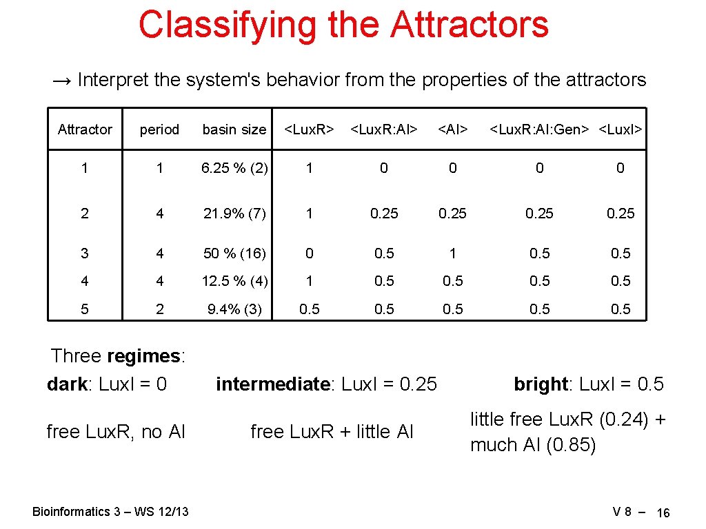
Classifying the Attractors → Interpret the system's behavior from the properties of the attractors Attractor period basin size <Lux. R> <Lux. R: AI> <AI> 1 1 6. 25 % (2) 1 0 0 2 4 21. 9% (7) 1 0. 25 3 4 50 % (16) 0 0. 5 1 0. 5 4 4 12. 5 % (4) 1 0. 5 5 2 9. 4% (3) 0. 5 0. 5 Three regimes: dark: Lux. I = 0 free Lux. R, no AI Bioinformatics 3 – WS 12/13 intermediate: Lux. I = 0. 25 free Lux. R + little AI <Lux. R: AI: Gen> <Lux. I> bright: Lux. I = 0. 5 little free Lux. R (0. 24) + much AI (0. 85) V 8 – 16

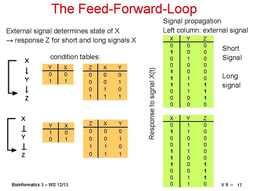
The Feed-Forward-Loop Signal propagation Left column: external signal External signal determines state of X → response Z for short and long signals X Y 0 1 Y 1 0 X 0 1 Bioinformatics 3 – WS 12/13 Z 0 0 0 1 Z 0 0 1 0 X 0 0 1 1 Y 0 1 0 1 Response to signal X(t) condition tables: X 0 1 0 0 1 1 1 0 0 0 Y 0 0 1 1 1 0 0 Z 0 0 0 1 1 1 0 X 0 1 0 0 1 1 1 0 0 0 Y 1 1 0 0 0 1 1 Z 0 0 0 1 1 1 0 Short Signal Long signal V 8 – 17

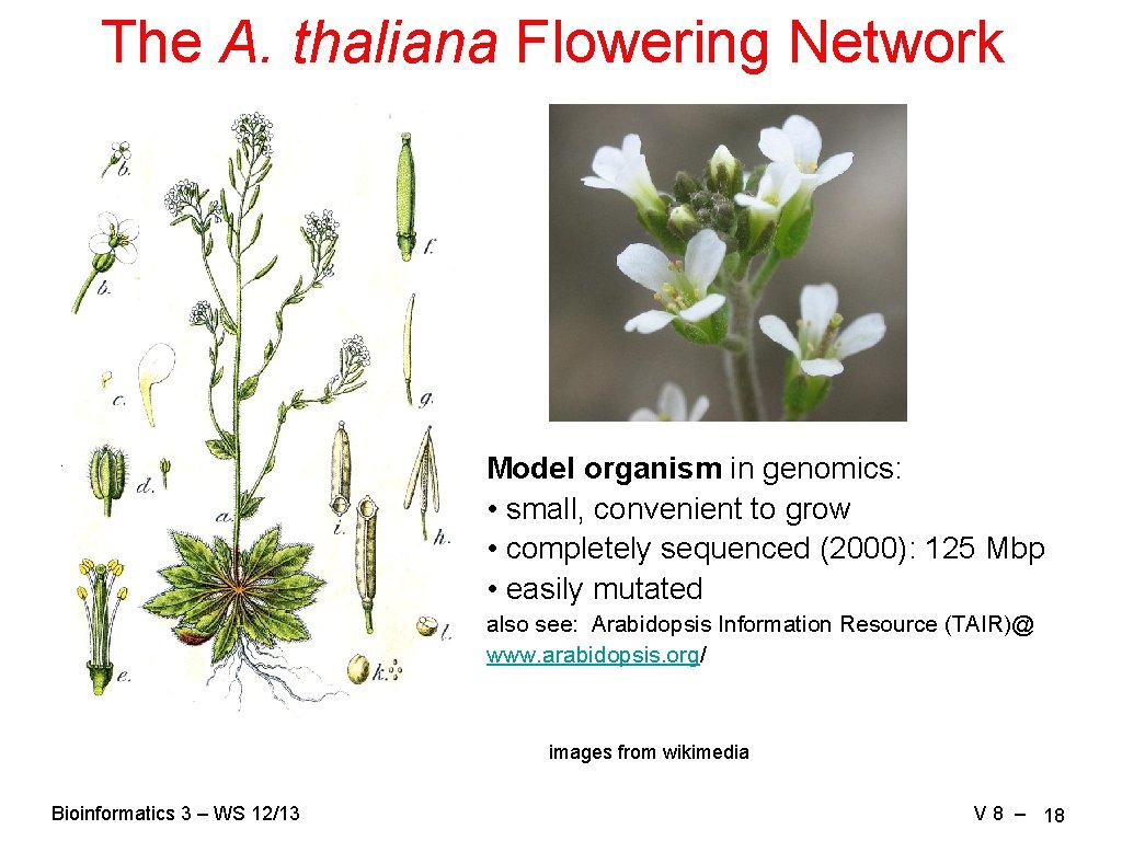
The A. thaliana Flowering Network Model organism in genomics: • small, convenient to grow • completely sequenced (2000): 125 Mbp • easily mutated also see: Arabidopsis Information Resource (TAIR)@ www. arabidopsis. org/ images from wikimedia Bioinformatics 3 – WS 12/13 V 8 – 18

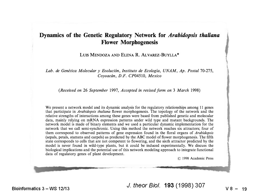
Bioinformatics 3 – WS 12/13 J. theor Biol. 193 (1998) 307 V 8 – 19

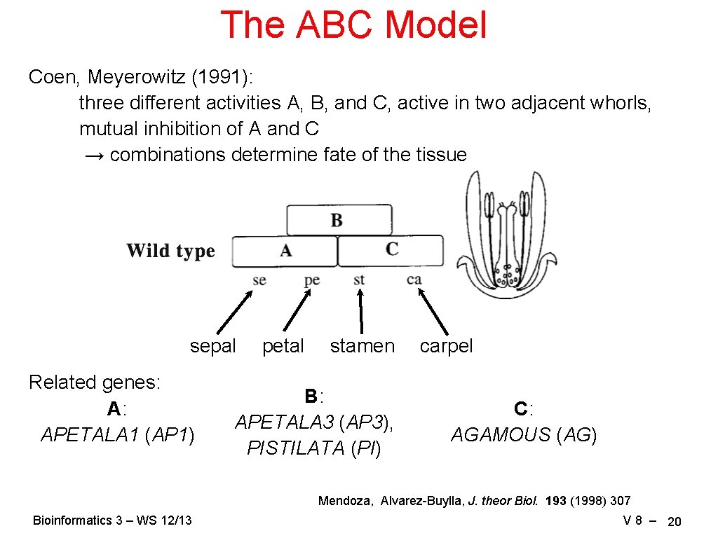
The ABC Model Coen, Meyerowitz (1991): three different activities A, B, and C, active in two adjacent whorls, mutual inhibition of A and C → combinations determine fate of the tissue sepal Related genes: A: APETALA 1 (AP 1) petal stamen B: APETALA 3 (AP 3), PISTILATA (PI) carpel C: AGAMOUS (AG) Mendoza, Alvarez-Buylla, J. theor Biol. 193 (1998) 307 Bioinformatics 3 – WS 12/13 V 8 – 20

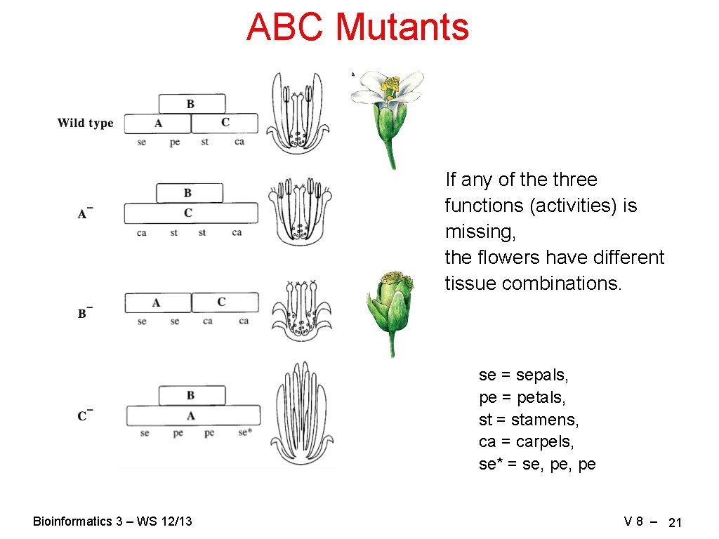
ABC Mutants If any of the three functions (activities) is missing, the flowers have different tissue combinations. se = sepals, pe = petals, st = stamens, ca = carpels, se* = se, pe Bioinformatics 3 – WS 12/13 V 8 – 21

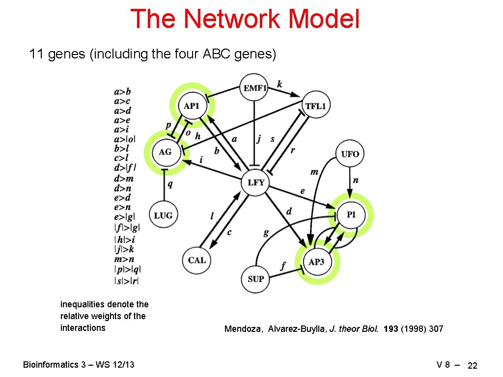
The Network Model 11 genes (including the four ABC genes) inequalities denote the relative weights of the interactions Bioinformatics 3 – WS 12/13 Mendoza, Alvarez-Buylla, J. theor Biol. 193 (1998) 307 V 8 – 22

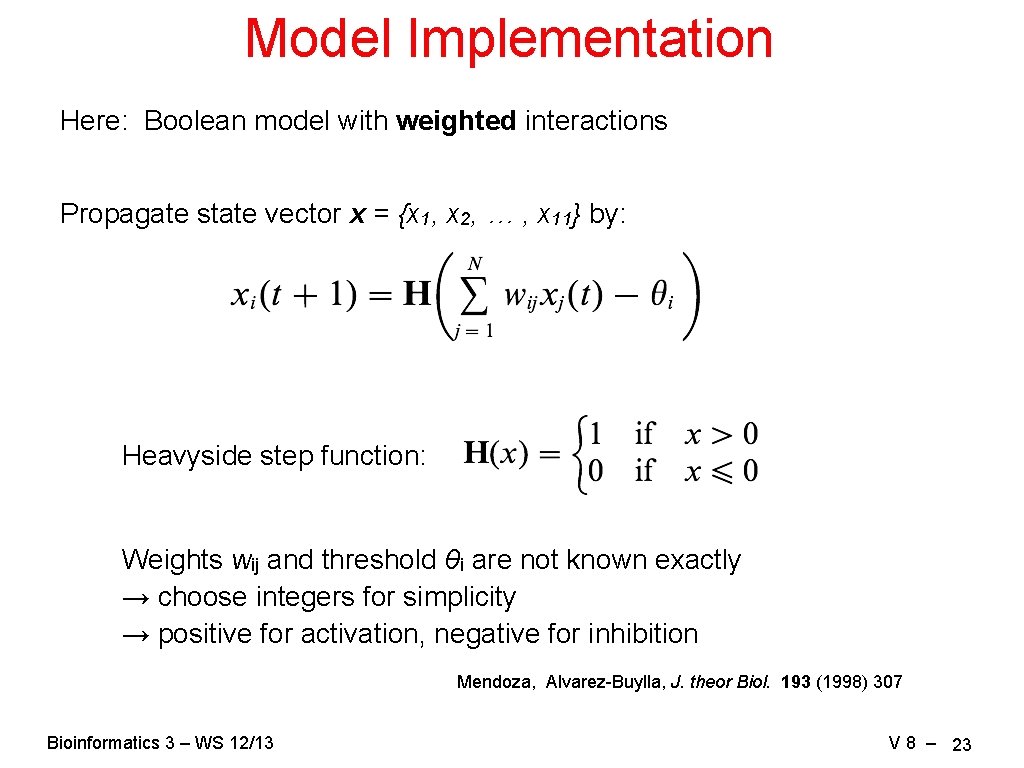
Model Implementation Here: Boolean model with weighted interactions Propagate state vector x = {x 1, x 2, … , x 11} by: Heavyside step function: Weights wij and threshold θi are not known exactly → choose integers for simplicity → positive for activation, negative for inhibition Mendoza, Alvarez-Buylla, J. theor Biol. 193 (1998) 307 Bioinformatics 3 – WS 12/13 V 8 – 23

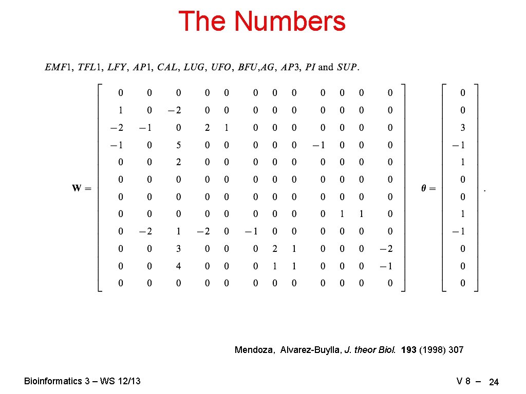
The Numbers Mendoza, Alvarez-Buylla, J. theor Biol. 193 (1998) 307 Bioinformatics 3 – WS 12/13 V 8 – 24

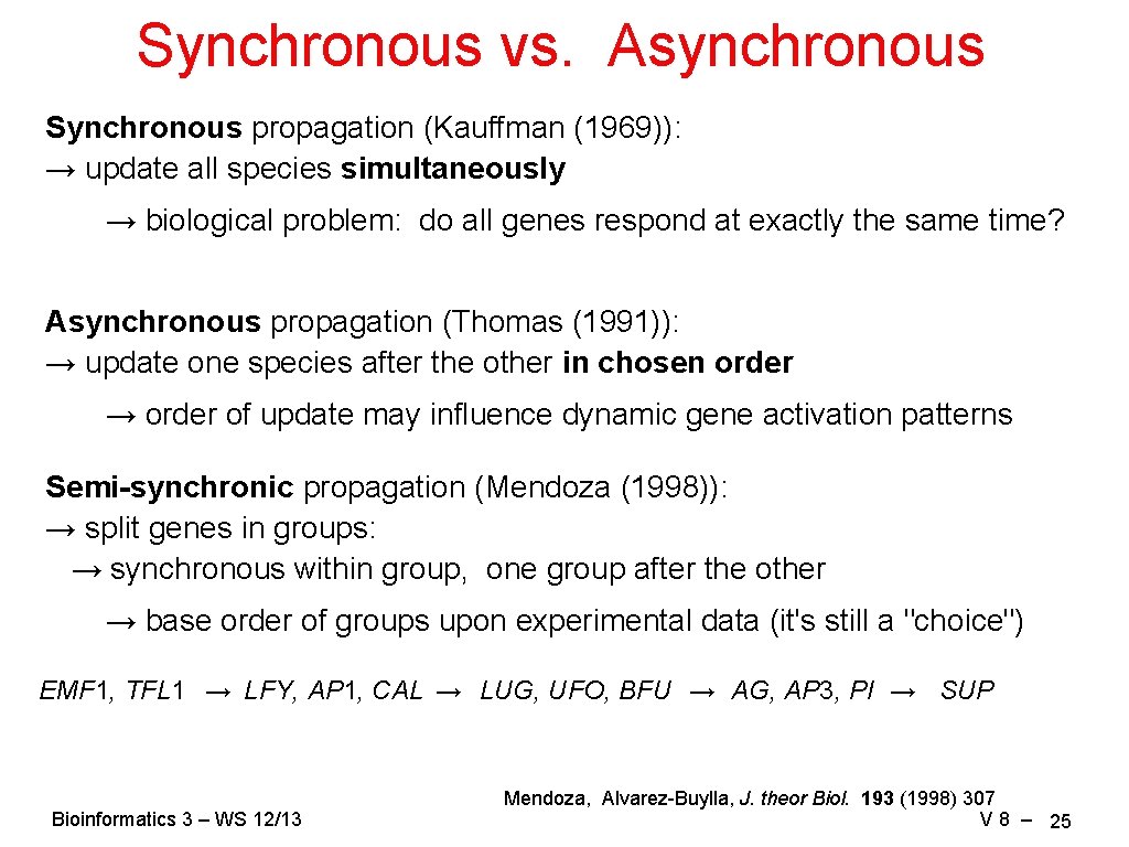
Synchronous vs. Asynchronous Synchronous propagation (Kauffman (1969)): → update all species simultaneously → biological problem: do all genes respond at exactly the same time? Asynchronous propagation (Thomas (1991)): → update one species after the other in chosen order → order of update may influence dynamic gene activation patterns Semi-synchronic propagation (Mendoza (1998)): → split genes in groups: → synchronous within group, one group after the other → base order of groups upon experimental data (it's still a "choice") EMF 1, TFL 1 → LFY, AP 1, CAL → LUG, UFO, BFU → AG, AP 3, PI → SUP Bioinformatics 3 – WS 12/13 Mendoza, Alvarez-Buylla, J. theor Biol. 193 (1998) 307 V 8 – 25

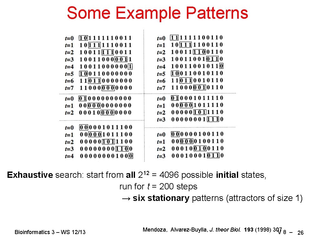
Some Example Patterns Exhaustive search: start from all 212 = 4096 possible initial states, run for t = 200 steps → six stationary patterns (attractors of size 1) Bioinformatics 3 – WS 12/13 Mendoza, Alvarez-Buylla, J. theor Biol. 193 (1998) 307 V 8 – 26

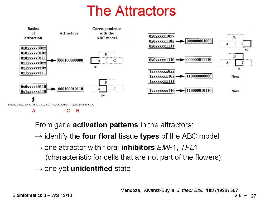
The Attractors A C B From gene activation patterns in the attractors: → identify the four floral tissue types of the ABC model → one attractor with floral inhibitors EMF 1, TFL 1 (characteristic for cells that are not part of the flowers) → one yet unidentified state Bioinformatics 3 – WS 12/13 Mendoza, Alvarez-Buylla, J. theor Biol. 193 (1998) 307 V 8 – 27

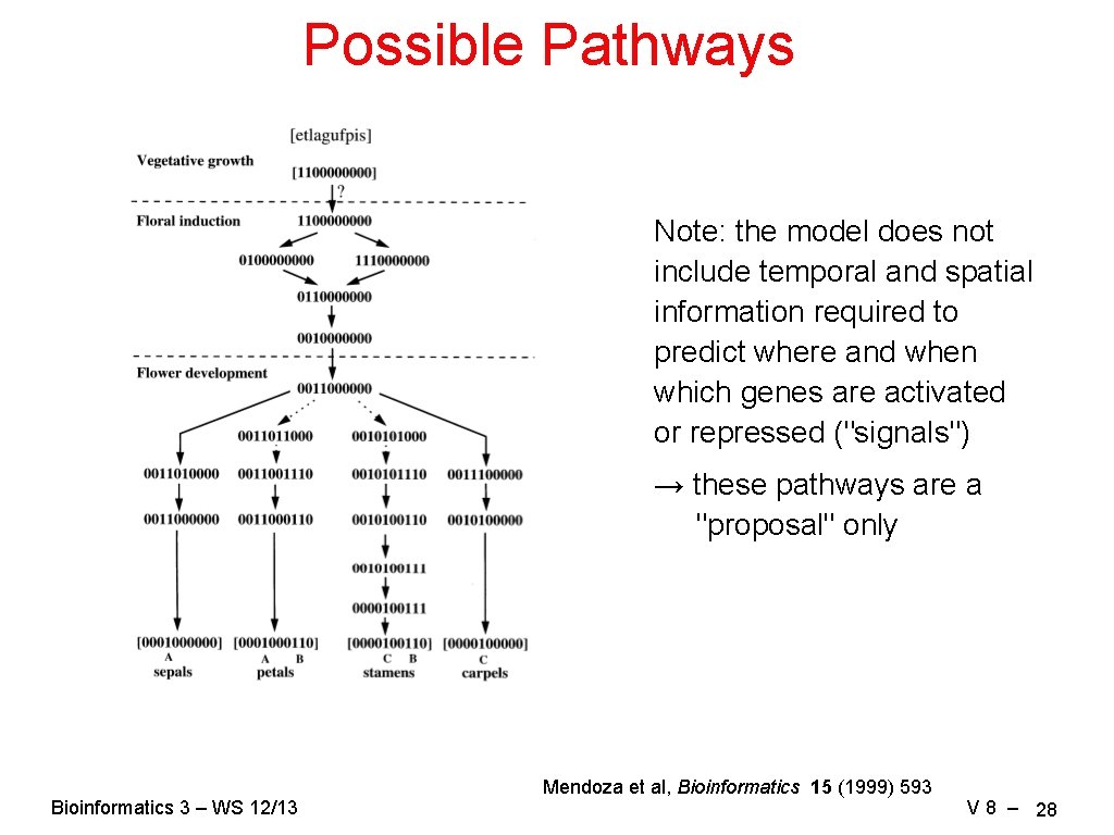
Possible Pathways Note: the model does not include temporal and spatial information required to predict where and when which genes are activated or repressed ("signals") → these pathways are a "proposal" only Bioinformatics 3 – WS 12/13 Mendoza et al, Bioinformatics 15 (1999) 593 V 8 – 28

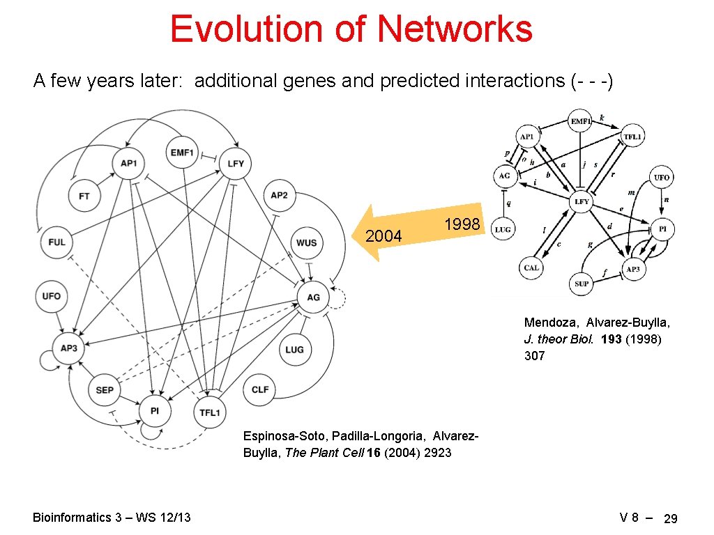
Evolution of Networks A few years later: additional genes and predicted interactions (- - -) 2004 1998 Mendoza, Alvarez-Buylla, J. theor Biol. 193 (1998) 307 Espinosa-Soto, Padilla-Longoria, Alvarez. Buylla, The Plant Cell 16 (2004) 2923 Bioinformatics 3 – WS 12/13 V 8 – 29

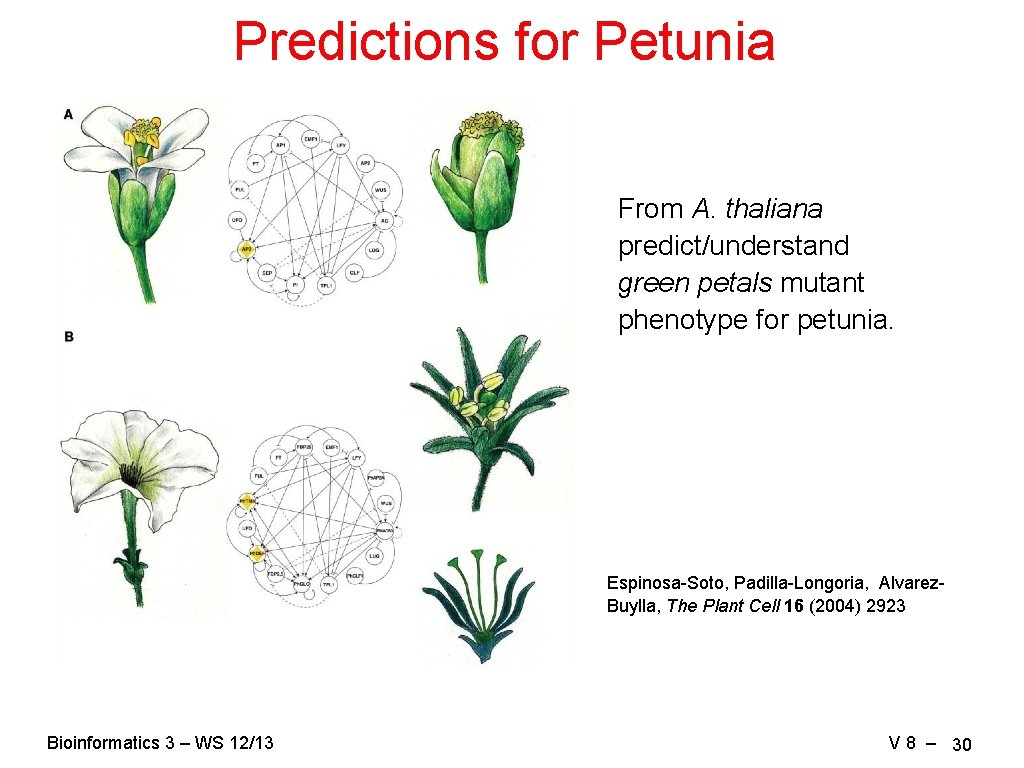
Predictions for Petunia From A. thaliana predict/understand green petals mutant phenotype for petunia. Espinosa-Soto, Padilla-Longoria, Alvarez. Buylla, The Plant Cell 16 (2004) 2923 Bioinformatics 3 – WS 12/13 V 8 – 30

What is it Worth? Generally: → quality of the results depends on the quality of the model → quality of the model depends on the quality of the assumptions Assumptions for the Boolean network description: ( • subset of the species considered → reduced system state space) • only discrete density levels • conditional yes–no causality → dynamic balances lost, reduced to oscillations → no continuous processes • discretized propagation steps → timing of concurrent paths? "You get what you pay for" Bioinformatics 3 – WS 12/13 V 8 – 31

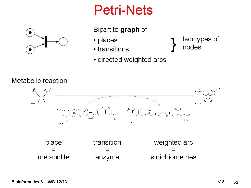
Petri-Nets Bipartite graph of } • places • transitions two types of nodes • directed weighted arcs Metabolic reaction: place = metabolite Bioinformatics 3 – WS 12/13 transition = enzyme weighted arc = stoichiometries V 8 – 32

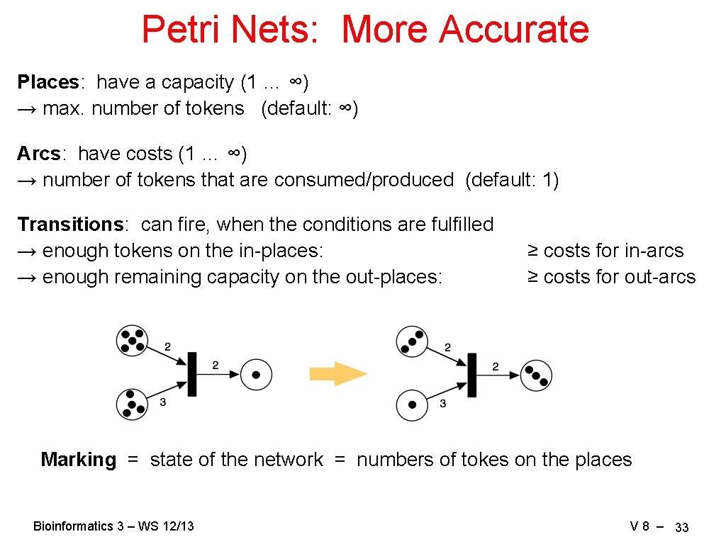
Petri Nets: More Accurate Places: have a capacity (1 … ∞) → max. number of tokens (default: ∞) Arcs: have costs (1 … ∞) → number of tokens that are consumed/produced (default: 1) Transitions: can fire, when the conditions are fulfilled → enough tokens on the in-places: → enough remaining capacity on the out-places: ≥ costs for in-arcs ≥ costs for out-arcs Marking = state of the network = numbers of tokes on the places Bioinformatics 3 – WS 12/13 V 8 – 33

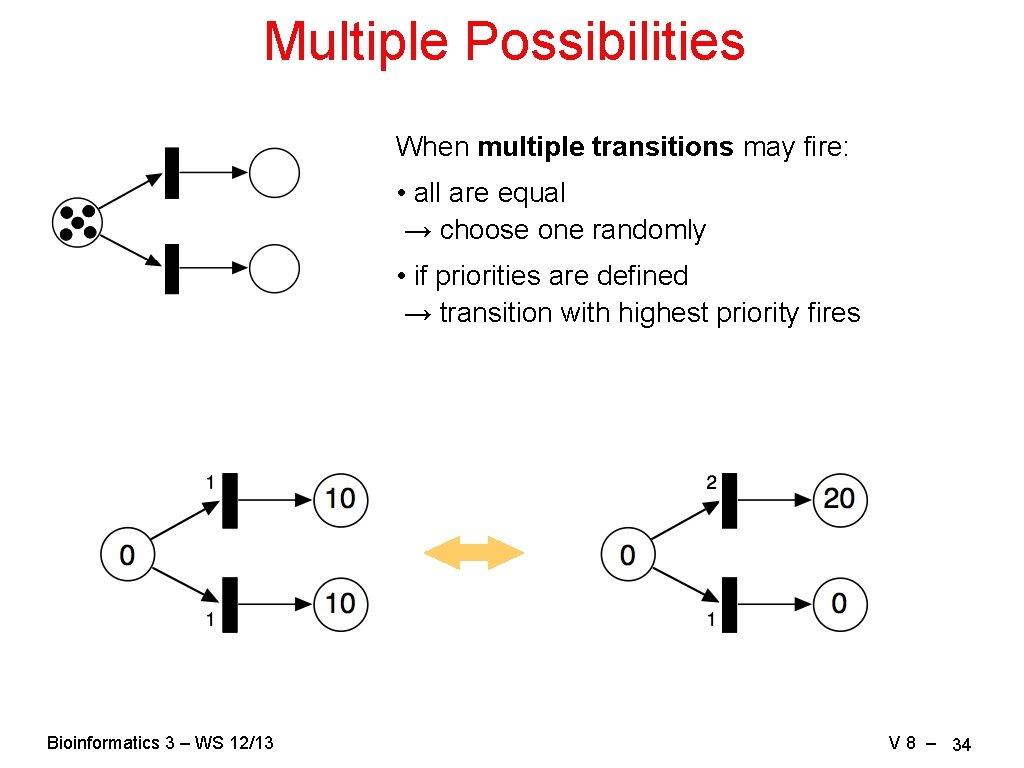
Multiple Possibilities When multiple transitions may fire: • all are equal → choose one randomly • if priorities are defined → transition with highest priority fires Bioinformatics 3 – WS 12/13 V 8 – 34

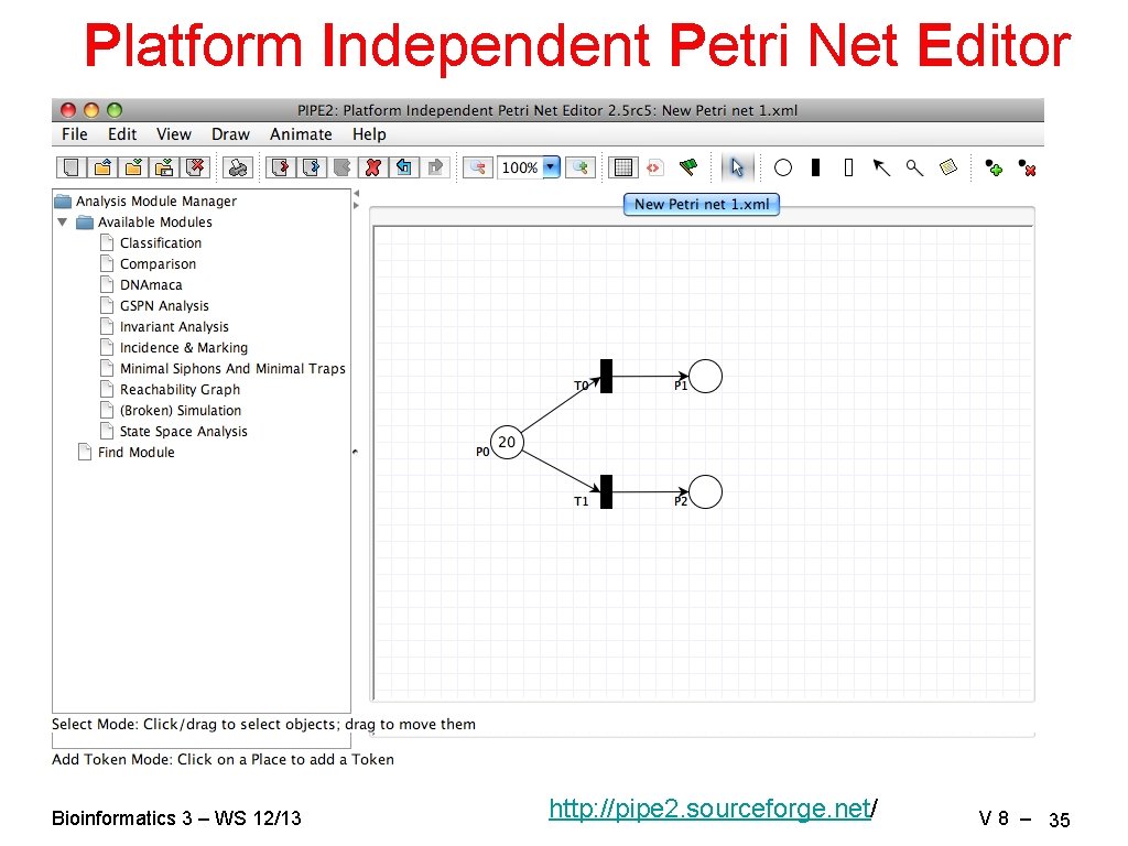
Platform Independent Petri Net Editor Bioinformatics 3 – WS 12/13 http: //pipe 2. sourceforge. net/ V 8 – 35

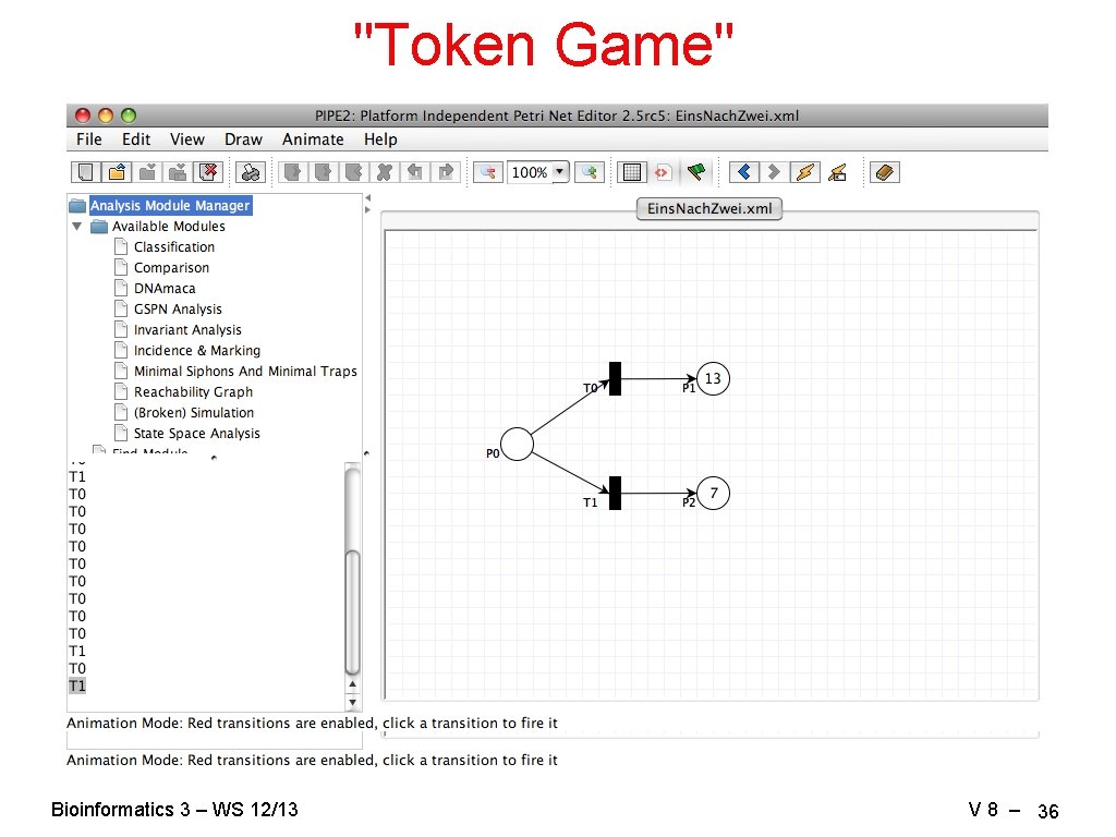
"Token Game" Bioinformatics 3 – WS 12/13 V 8 – 36

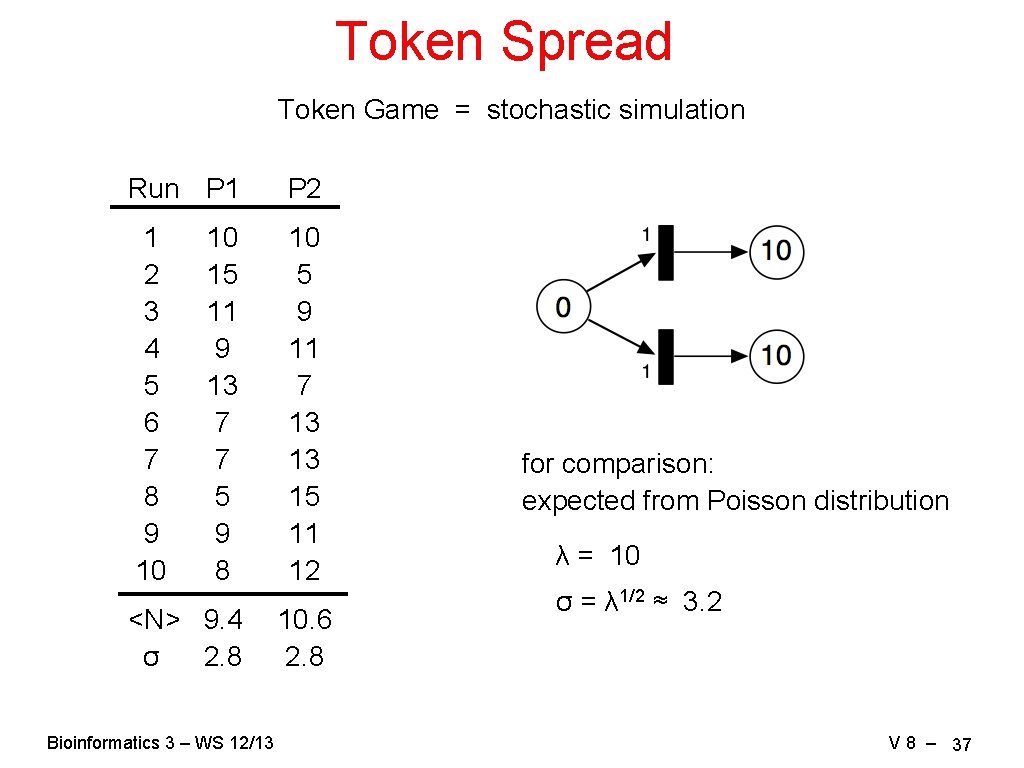
Token Spread Token Game = stochastic simulation Run P 1 P 2 1 2 3 4 5 6 7 8 9 10 10 5 9 11 7 13 13 15 11 12 10 15 11 9 13 7 7 5 9 8 <N> 9. 4 σ 2. 8 Bioinformatics 3 – WS 12/13 10. 6 2. 8 for comparison: expected from Poisson distribution λ = 10 σ = λ 1/2 ≈ 3. 2 V 8 – 37

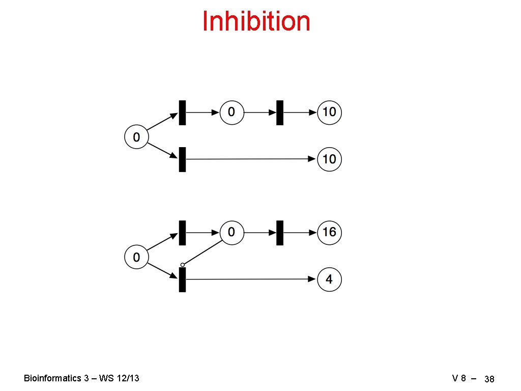
Inhibition Bioinformatics 3 – WS 12/13 V 8 – 38

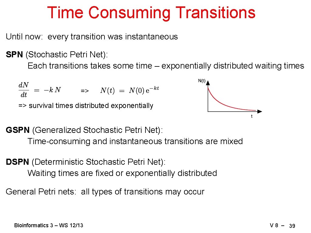
Time Consuming Transitions Until now: every transition was instantaneous SPN (Stochastic Petri Net): Each transitions takes some time – exponentially distributed waiting times => => survival times distributed exponentially GSPN (Generalized Stochastic Petri Net): Time-consuming and instantaneous transitions are mixed DSPN (Deterministic Stochastic Petri Net): Waiting times are fixed or exponentially distributed General Petri nets: all types of transitions may occur Bioinformatics 3 – WS 12/13 V 8 – 39

Analysis "Token Game" simulations → phenomenological: what happens, does the model work? → stationary states? (we're stuck…) → periodic orbits? → relative probabilities of certain states? "State space analysis" → average number of tokens, distributions, throughputs → reachability of markings (states) → liveliness → deadlocks, traps, siphons Bioinformatics 3 – WS 12/13 V 8 – 40

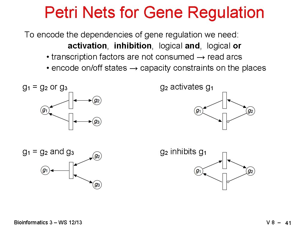
Petri Nets for Gene Regulation To encode the dependencies of gene regulation we need: activation, inhibition, logical and, logical or • transcription factors are not consumed → read arcs • encode on/off states → capacity constraints on the places g 1 = g 2 or g 3 g 2 activates g 1 = g 2 and g 3 g 2 inhibits g 1 Bioinformatics 3 – WS 12/13 V 8 – 41

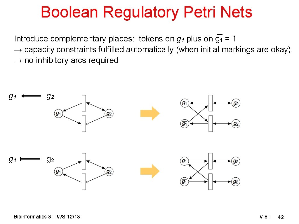
Boolean Regulatory Petri Nets Introduce complementary places: tokens on g 1 plus on g 1 = 1 → capacity constraints fulfilled automatically (when initial markings are okay) → no inhibitory arcs required g 1 g 2 Bioinformatics 3 – WS 12/13 V 8 – 42

Reverse Engineering Networks Problem: "Find the network that explains the biological processes!" → usually too ambitious Experiments: co-expression data → co-regulation of different genes (correlation or direct interaction? ) → time-series of individual genes Strategies: "Find all networks that are compatible with the experiments" → combinatorial explosion, usually too many candidates → does not work… "Find one network that is compatible with the experiments" → solvable task, but how good is this network? → does not work… "Find some networks that are compatible with the experiments" → algorithms exist, need heuristics (experience) to assess coverage → does work… Bioinformatics 3 – WS 12/13 V 8 – 43

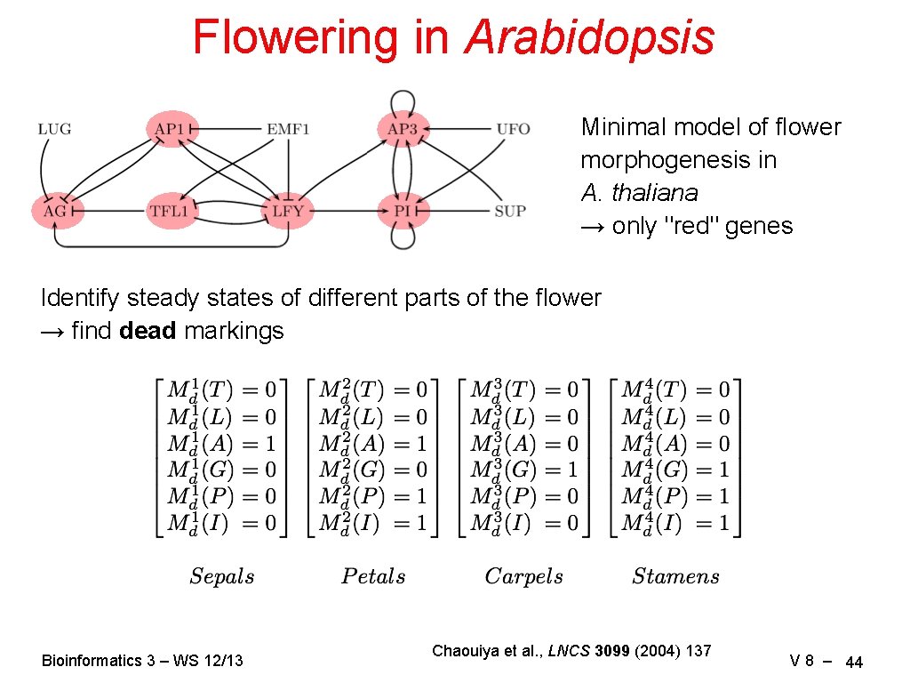
Flowering in Arabidopsis Minimal model of flower morphogenesis in A. thaliana → only "red" genes Identify steady states of different parts of the flower → find dead markings Bioinformatics 3 – WS 12/13 Chaouiya et al. , LNCS 3099 (2004) 137 V 8 – 44

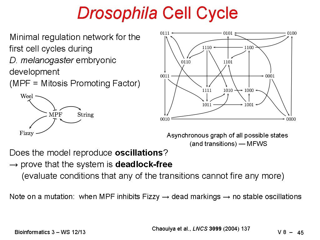
Drosophila Cell Cycle Minimal regulation network for the first cell cycles during D. melanogaster embryonic development (MPF = Mitosis Promoting Factor) Asynchronous graph of all possible states (and transitions) — MFWS Does the model reproduce oscillations? → prove that the system is deadlock-free (evaluate conditions that any of the transitions cannot fire any more) Note on a mutation: when MPF inhibits Fizzy → dead markings → no stable oscillations Bioinformatics 3 – WS 12/13 Chaouiya et al. , LNCS 3099 (2004) 137 V 8 – 45

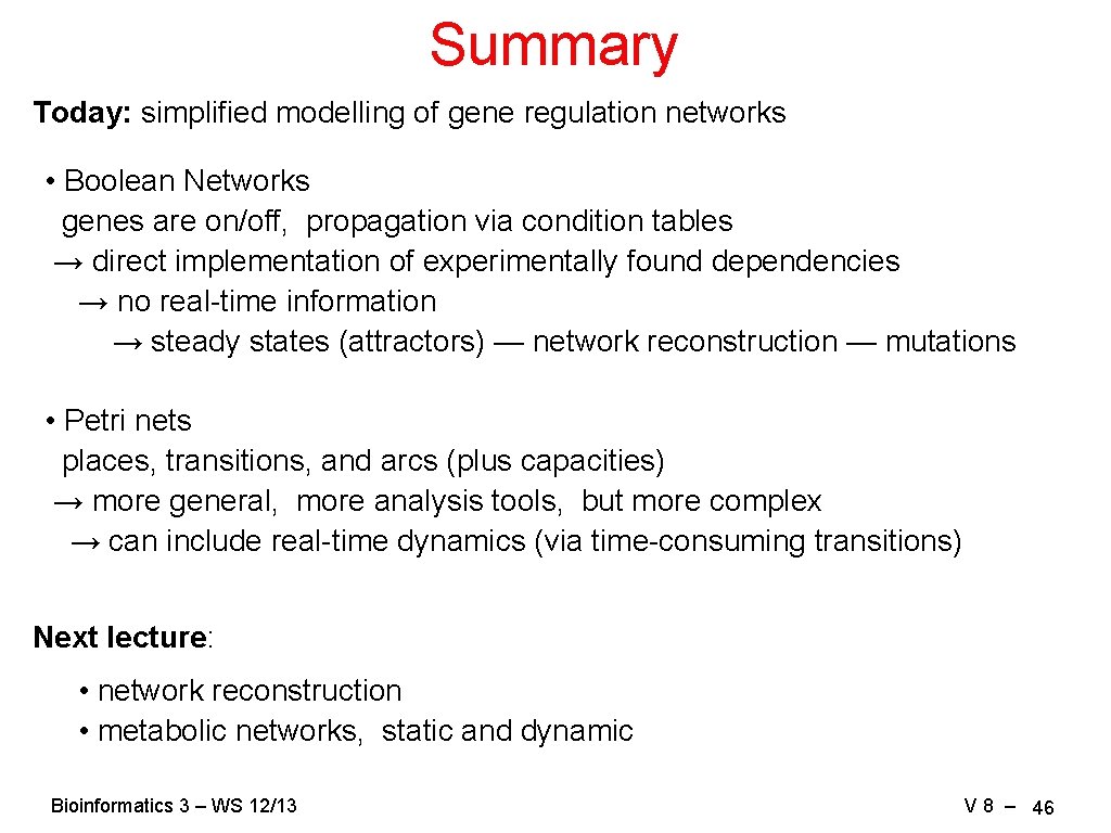
Summary Today: simplified modelling of gene regulation networks • Boolean Networks genes are on/off, propagation via condition tables → direct implementation of experimentally found dependencies → no real-time information → steady states (attractors) — network reconstruction — mutations • Petri nets places, transitions, and arcs (plus capacities) → more general, more analysis tools, but more complex → can include real-time dynamics (via time-consuming transitions) Next lecture: • network reconstruction • metabolic networks, static and dynamic Bioinformatics 3 – WS 12/13 V 8 – 46