Biodiversity Mapping Approaches Team Gary Beauvais Pat Comer

Biodiversity Mapping Approaches Team: Gary Beauvais, Pat Comer, Jon Hak, Rickie White, Jennifer Nichols, Jim Morefield, Bruce Stein, Larry Master Nature. Serve Western Regional Conference April 2008

Why a Biodiversity Mapping Approaches Team? Nature. Serve and the network recognize that: • Methods and products for representing Biodiversity data as EOs worked (in many instances) • With improvements in technology and biodiversity data, additional mapping products are available and requested by clients and partners • Core heritage methodology and technologies have not always kept pace
 As a result: • Network programs, along with some at central")
Why BMAT? (continued) As a result: • Network programs, along with some at central Nature. Serve, have independently developed spatial techniques, technologies, and products • This has led to some “fragmentation” across the network as programs responded differently to new requests and opportunities • This challenges our biggest strength: consistent methodology and products across the Nature. Serve network
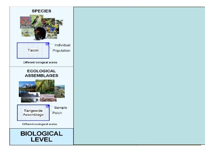
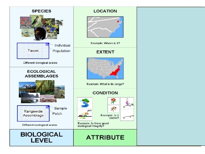
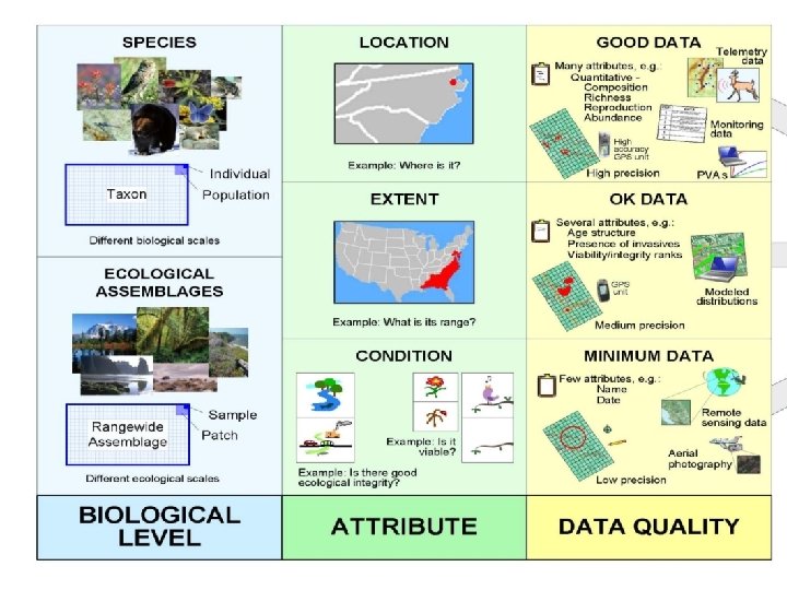

The Matrix: Species Min. data Individual Location Extent Condition Pop. segment Location Extent Condition Taxon Location Extent Condition OK data Good data

OK Data Population segment : Extent Data: georeferenced observations w/ good attribution and map precision; some observations clustered in time and space; most observations opportunistic, some from structured inventories; some knowledge of movement distances and habitat use Map methods: basic buffering of observations; minimum convex polygon; EO spatial methods; deductive distribution modeling and mapping; basic spatial statistics Example output: polygonal pop. segment map based on appropriate extrapolation of clustered observations

Mapping Approaches Matrix Analysis Additional information was added to the matrix for identifying priority mapping approaches • Examples of user stories • Utility of the approach to Nature. Serve • How important is this spatial data to conservation? • How well does the network produce the info? • Are effective and efficient methods available that are realistic to implement? • Are these methods implemented consistently across the network?

Ecology Field Methods Community EO Field inventory to document Community Occurrences

Occurrence Specifications: Minimum Patch size, Separation Distance, and Barriers 5 0. 3 km 10 Barrier 2 10 2 0. 5 km 10

Observations, Occurrences, and Maps Field Samples to Remotelysensed Data, to EOs, Community EO

The Matrix: Ecological Elements Min. data Observation Location Extent Condition Location Patch Extent Condition Location Rangewide Distribution Extent Condition OK data Good data
")
Observation Data Colorado Plateau Blackbrush-Morman Tea Shrubland (ecological system)
 of an")
User Story: Building an inductive model-based distribution (and accuracy assessment of map) of an ecological concept and needs individual georeferenced data points (individual samples such as plots) on which to base analysis and map. OK Data: a georeferenced sample point (within 25 -100 m radius) usually collected via a structured sample design (and therefore sample may be part of a larger cluster of samples within a study area); usually recent but can be historic. Sample Observation: Attributes: name of point/plot, data on biological composition, basic environmental data, labeled with standard classification concept; Sample should be recently collected but may be older. Location Map methods: basic sample mapping with lat/long, modified polygon representation on map based on precision. Example product: point-based sample map (such as a point representing a plot) with precision, last observed date of sample, and name of standard classification concept.

The Matrix: Ecological Elements Min. data Observation Location Extent Condition Location Patch Extent Condition Location Rangewide Distribution Extent Condition OK data Good data

Lower Westwater 2000 Lower Westwater 1986 Sagebrush 5, 133 stems/acre Sagebrush 1, 240 stems/acre Lower Westwater 2005 Data from UT DNR Sagebrush 60 stems/acre

OK Data: a georeferenced polygonal representation of the full extent of the sample (usually a plot); Sample Observation: Condition Attributes: qualitative information (e. g. , from a photograph) typically available on assemblage composition, richness, age structure, or other ecological characters as well as some sample attributes that indirectly measure appropriate ecological characters. Landscape condition model may be applied to the region and values assigned to individual samples based on contextual land/water use attributes. Generic EO Rank criteria available to apply towards point with qualitative metrics defined Estimating condition: 1) establish basic rules for presence/absence, and other qualitative categories that could be derived from sample information to determine quality 2) append index score from landscape condition model to sample Map methods: map the sample location and color-code/label with EO Rank Example product: sample location or extent map w/ condition symbolized; moderate confidence

The Matrix: Ecological Elements Min. data Observation Location Extent Condition Location Patch Extent Condition Location Rangewide Distribution Extent Condition OK data Good data

Patch = traditional EO Community EO Field inventory to document Community Occurrences

Good Data Patch: Condition Data: EO Spec derived from type-specific EO spec applied to field based observation (often with additional field based delineation of boundaries); with evaluation of quality/condition based on established type-specific EO Rank spec and applied using a mix of remotely sensed and field based qualitative and quantitative metrics; with repeat measurement Estimating condition: apply updated quantitative metrics derived from type-specific EO Rank criteria Map methods: as above, but applying EO Rank spec criteria for size, biotic condition, and landscape context; and capturing trend. Example product: EO map(s) with condition estimate(s) derived over time, of high confidence, due to good quality inputs and precise evaluation criteria.

The Matrix: Ecological Elements Min. data Observation Location Extent Condition Location Patch Extent Condition Location Rangewide Distribution Extent Condition OK data Good data

The Matrix: Ecological Elements Min. data Observation Location Extent Condition Location Patch Extent Condition Location Rangewide Distribution Extent Condition OK data Good data
")
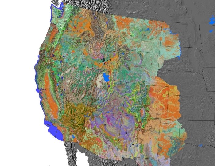
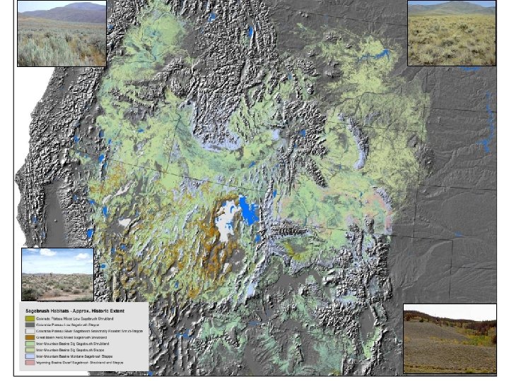
Mapped Distribution Colorado Plateau Blackbrush-Morman Tea Shrubland (ecological system)
")
Inputs for Inventory Field sample Colorado Plateau Blackbrush-Morman Tea Shrubland (ecological system)

Modeling Landscape Condition

Occurrence Specifications: Minimum Patch size, Separation Distance, and Barriers 5 0. 3 km 10 Barrier 2 10 2 0. 5 km 10

Processing Mapped Data – a Phased Approach to EO delineation Barriers Inserted Separation Distance Applied ‘Proto-EO’ Identified

OK Data: EO Rank based on generic criteria and/or application of spatial analysis and/or model of landscape condition. Patch: Condition Estimating condition: evaluation of quality/condition based on established group EO Rank spec and applied using a mix of remotely sensed and field based qualitative metrics Map methods: as above, but applying EO Rank spec criteria for size, biotic condition, and landscape context Example product: EO map with condition estimate, of moderate/high confidence, due to moderate/good quality inputs and evaluation criteria (from one or more points in time)

The Matrix: Ecological Elements Min. data Observation Location Extent Condition Location Patch Extent Condition Location Rangewide Distribution Extent Condition OK data Good data

NVC Class

NVC Subclass

NVC Formation

NVC Division

NVC Macrogroup

NVC Group

Range Map e. g. , selected ECOMAP subsections Colorado Plateau Blackbrush-Morman Tea Shrubland

Good Data Rangewide: Location Data: Distribution derived from mapped/modeled mapping and subsequent attribution by moderate/local-sized spatial unit, like TNC/EPA ecoregional subunits or subwatersheds (14 digit HUs or stream segmentsheds). May depict multiple time periods. Map Methods: highlighted sub-ecoregio/watershed distribution map using mapped data to derive attribute table. Example Products: highlighted sub-ecoregion/watershed distribution map (with trends over time)

BMAT Findings 1. Most spatial information types are based on observations, so these need to be an important focus of program data management 2. For species, the most important information for conservation and management is extent and condition of population segments, which reaffirms the centrality of EOs in our methodology 3. Ecological elements range from rare to common (i. e. , common elements are the “coarse filter”), and the latter brings special mapping considerations

More BMAT Findings 4. Ecological aspects of Biodiversity spatial data are equally based on observations (samples) and maps which, in various combinations, can be used to derive EOs 5. There appears to be a natural “crossover” between the fundamental species and ecology categories in the network’s mapping activities. . .
 • Range")
Ecology Spatial Data Categories • Observation • Occurrence • Map (moderate/high resolution) • Range Map (low resolution)
- Slides: 44