Binomial Probability Distribution For the binomial distribution P
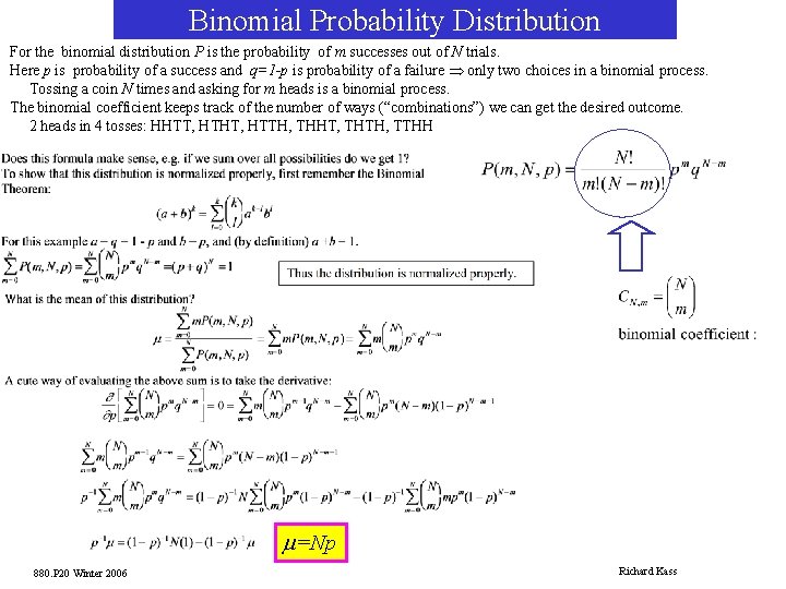
Binomial Probability Distribution For the binomial distribution P is the probability of m successes out of N trials. Here p is probability of a success and q=1 -p is probability of a failure Þ only two choices in a binomial process. Tossing a coin N times and asking for m heads is a binomial process. The binomial coefficient keeps track of the number of ways (“combinations”) we can get the desired outcome. 2 heads in 4 tosses: HHTT, HTHT, HTTH, THHT, THTH, TTHH m=Np 880. P 20 Winter 2006 Richard Kass
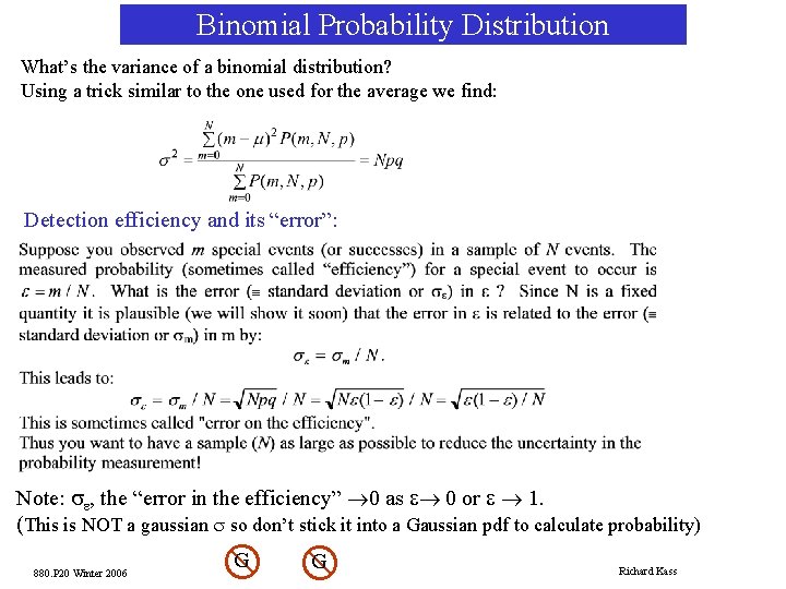
Binomial Probability Distribution What’s the variance of a binomial distribution? Using a trick similar to the one used for the average we find: Detection efficiency and its “error”: Note: se, the “error in the efficiency” ® 0 as e® 0 or e ® 1. (This is NOT a gaussian s so don’t stick it into a Gaussian pdf to calculate probability) 880. P 20 Winter 2006 G G x x Richard Kass
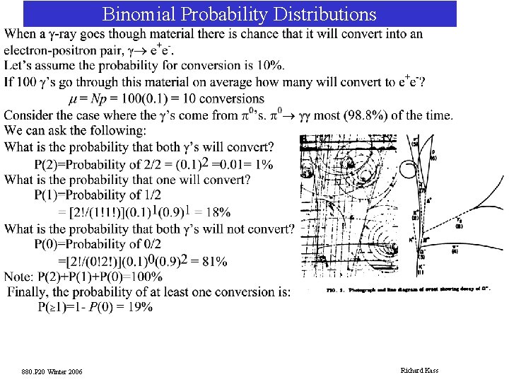
Binomial Probability Distributions 880. P 20 Winter 2006 Richard Kass
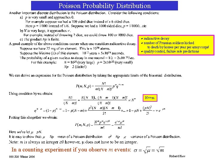
Poisson Probability Distribution aradioactive decay anumber of Prussian soldiers kicked to death by horses per year per army corps! aquality control, failure rate predictions N>>m In a counting experiment if you observe m events: 880. P 20 Winter 2006 Richard Kass
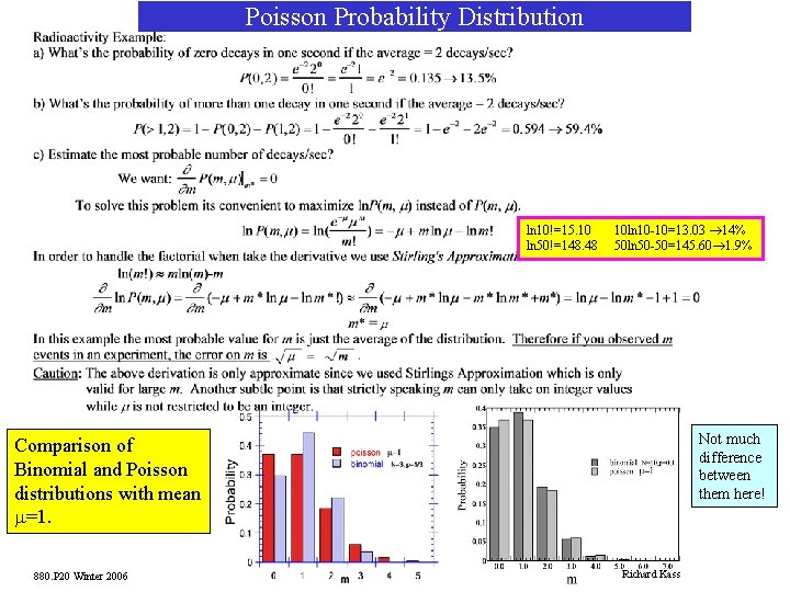
Poisson Probability Distribution ln 10!=15. 10 ln 50!=148. 48 10 ln 10 -10=13. 03 ® 14% 50 ln 50 -50=145. 60® 1. 9% Not much difference between them here! Comparison of Binomial and Poisson distributions with mean m=1. 880. P 20 Winter 2006 Richard Kass
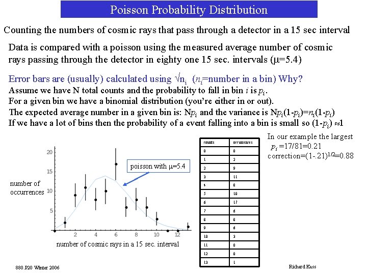
Poisson Probability Distribution Counting the numbers of cosmic rays that pass through a detector in a 15 sec interval Data is compared with a poisson using the measured average number of cosmic rays passing through the detector in eighty one 15 sec. intervals (m=5. 4) Error bars are (usually) calculated using Öni (ni=number in a bin) Why? Assume we have N total counts and the probability to fall in bin i is pi. For a given bin we have a binomial distribution (you’re either in or out). The expected average number in a given bin is: Npi and the variance is Npi(1 -pi)=ni(1 -pi) If we have a lot of bins then the probability of a event falling into a bin is small so (1 -pi) » 1 poisson with m=5. 4 number of occurrences number of cosmic rays in a 15 sec. interval 880. P 20 Winter 2006 counts occurrences 0 0 1 2 2 9 3 11 4 8 5 10 6 17 7 6 8 8 9 6 10 3 11 0 12 0 13 1 In our example the largest pi =17/81=0. 21 correction=(1 -. 21)1/2=0. 88 Richard Kass
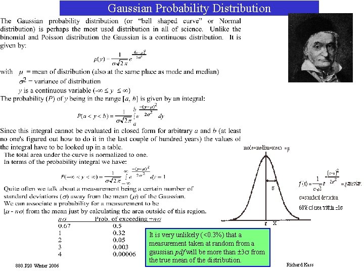
Gaussian Probability Distribution x 880. P 20 Winter 2006 It is very unlikely (<0. 3%) that a measurement taken at random from a gaussian pdf will be more than ± 3 s from the true mean of the distribution. Richard Kass
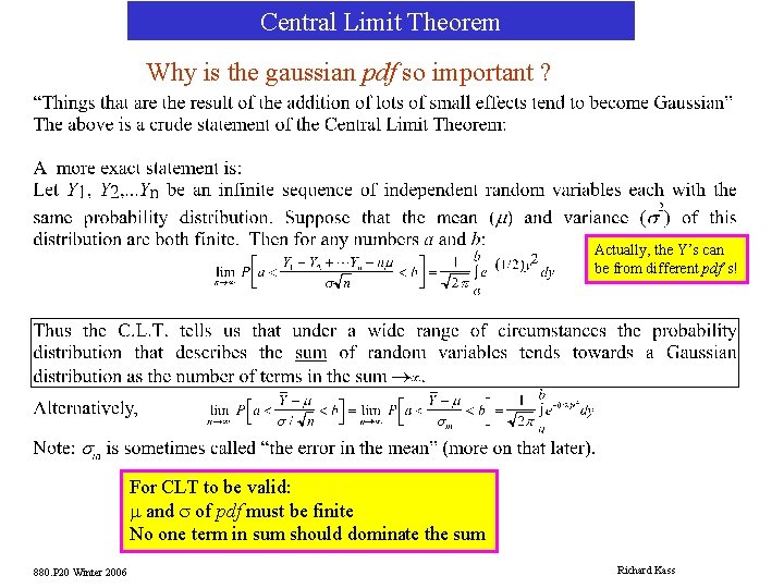
Central Limit Theorem Why is the gaussian pdf so important ? Actually, the Y’s can be from different pdf’s! For CLT to be valid: m and s of pdf must be finite No one term in sum should dominate the sum 880. P 20 Winter 2006 Richard Kass
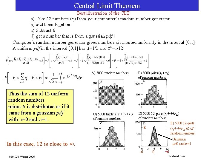
Central Limit Theorem Best illustration of the CLT. a) Take 12 numbers (ri) from your computer’s random number generator b) add them together c) Subtract 6 d) get a number that is from a gaussian pdf ! Computer’s random number generator gives numbers distributed uniformly in the interval [0, 1] A uniform pdf in the interval [0, 1] has m=1/2 and s 2=1/12 A) 5000 random numbers Thus the sum of 12 uniform random numbers minus 6 is distributed as if it came from a gaussian pdf with m=0 and s=1. C) 5000 triplets (r 1+ r 2+ r 3) of random numbers B) 5000 pairs (r 1+ r 2) of random numbers D) 5000 12 -plets (r 1+ ++r 12) of random numbers. E) 5000 12 -plets E (r + ++r -6) of 1 12 random numbers. Gaussian m=0 and s=1 In this case, 12 is close to ¥. -6 880. P 20 Winter 2006 0 +6 Richard Kass
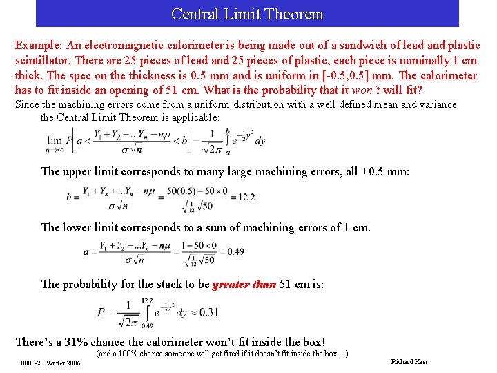
Central Limit Theorem Example: An electromagnetic calorimeter is being made out of a sandwich of lead and plastic scintillator. There are 25 pieces of lead and 25 pieces of plastic, each piece is nominally 1 cm thick. The spec on the thickness is 0. 5 mm and is uniform in [-0. 5, 0. 5] mm. The calorimeter has to fit inside an opening of 51 cm. What is the probability that it won’t will fit? Since the machining errors come from a uniform distribution with a well defined mean and variance the Central Limit Theorem is applicable: The upper limit corresponds to many large machining errors, all +0. 5 mm: The lower limit corresponds to a sum of machining errors of 1 cm. The probability for the stack to be greater than 51 cm is: There’s a 31% chance the calorimeter won’t fit inside the box! (and a 100% chance someone will get fired if it doesn’t fit inside the box…) 880. P 20 Winter 2006 Richard Kass
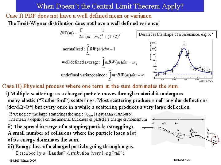
When Doesn’t the Central Limit Theorem Apply? Case I) PDF does not have a well defined mean or variance. The Breit-Wigner distribution does not have a well defined variance! Describes the shape of a resonance, e. g. K* Case II) Physical process where one term in the sum dominates the sum. i) Multiple scattering: as a charged particle moves through material it undergoes many elastic (“Rutherford”) scatterings. Most scattering produce small angular deflections (ds/d. W~q-4) but every once in a while a scattering produces a very large deflection. If we neglect the large scatterings the angle qplane is gaussian distributed. The mean q depends on the material thickness & particle’s charge & momentum ii) The spread in range of a stopping particle (straggling). A small number of collisions where the particle loses a lot of its energy dominates the sum. iii) Energy loss of a charged particle going through a gas. Described by a “Landau” distribution (very long “tail”). 880. P 20 Winter 2006 Richard Kass
- Slides: 11