BINOMIAL DISTRIBUTION The context The properties Notation Formula

BINOMIAL DISTRIBUTION • • • The context The properties Notation Formula Mean and variance

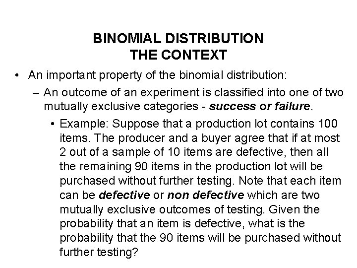
BINOMIAL DISTRIBUTION THE CONTEXT • An important property of the binomial distribution: – An outcome of an experiment is classified into one of two mutually exclusive categories - success or failure. • Example: Suppose that a production lot contains 100 items. The producer and a buyer agree that if at most 2 out of a sample of 10 items are defective, then all the remaining 90 items in the production lot will be purchased without further testing. Note that each item can be defective or non defective which are two mutually exclusive outcomes of testing. Given the probability that an item is defective, what is the probability that the 90 items will be purchased without further testing?

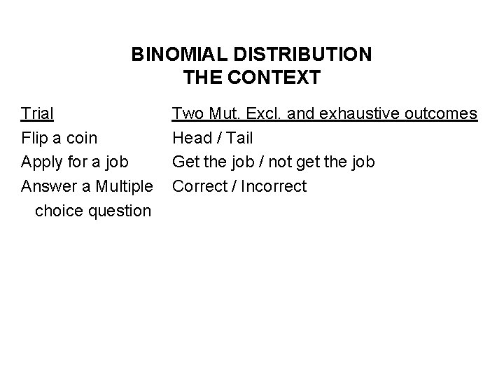
BINOMIAL DISTRIBUTION THE CONTEXT Trial Flip a coin Apply for a job Answer a Multiple choice question Two Mut. Excl. and exhaustive outcomes Head / Tail Get the job / not get the job Correct / Incorrect

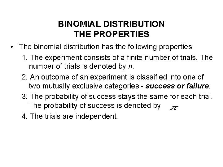
BINOMIAL DISTRIBUTION THE PROPERTIES • The binomial distribution has the following properties: 1. The experiment consists of a finite number of trials. The number of trials is denoted by n. 2. An outcome of an experiment is classified into one of two mutually exclusive categories - success or failure. 3. The probability of success stays the same for each trial. The probability of success is denoted by 4. The trials are independent.

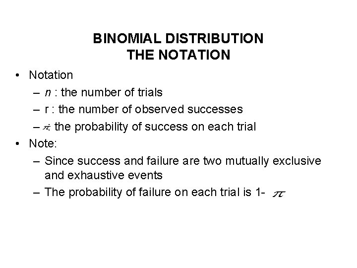
BINOMIAL DISTRIBUTION THE NOTATION • Notation – n : the number of trials – r : the number of observed successes – : the probability of success on each trial • Note: – Since success and failure are two mutually exclusive and exhaustive events – The probability of failure on each trial is 1 -

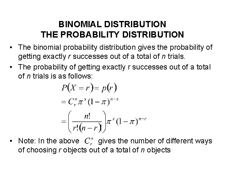
BINOMIAL DISTRIBUTION THE PROBABILITY DISTRIBUTION • The binomial probability distribution gives the probability of getting exactly r successes out of a total of n trials. • The probability of getting exactly r successes out of a total of n trials is as follows: • Note: In the above gives the number of different ways of choosing r objects out of a total of n objects

Example 1 • There are 5 parts to be checked. We are considering exactly r=2 defectives occurring in those parts. (see page 208). (i) How many ways two defectives can be found? (ii) Since the elementary event in each of these cases has probability. 00729, so what is the probability of getting exactly two defectives.

Example from page 209

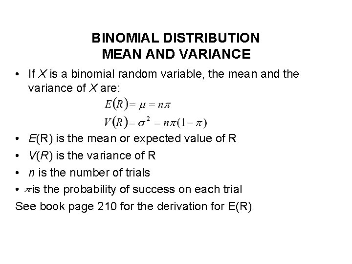
BINOMIAL DISTRIBUTION MEAN AND VARIANCE • If X is a binomial random variable, the mean and the variance of X are: • E(R) is the mean or expected value of R • V(R) is the variance of R • n is the number of trials • is the probability of success on each trial See book page 210 for the derivation for E(R)

Cumulative Probability and the Binomial Probability Table • When n is small, it is easy to compute binomial probabilities using a calculator • To ease the computational burden, the more common binomial probabilities have been tabled. • Such tables are usually constructed in terms of cumulative probabilities • A cumulative probability is found by summing the individual probability terms applicable to all levels of the random variable that fall at or below a specified point.

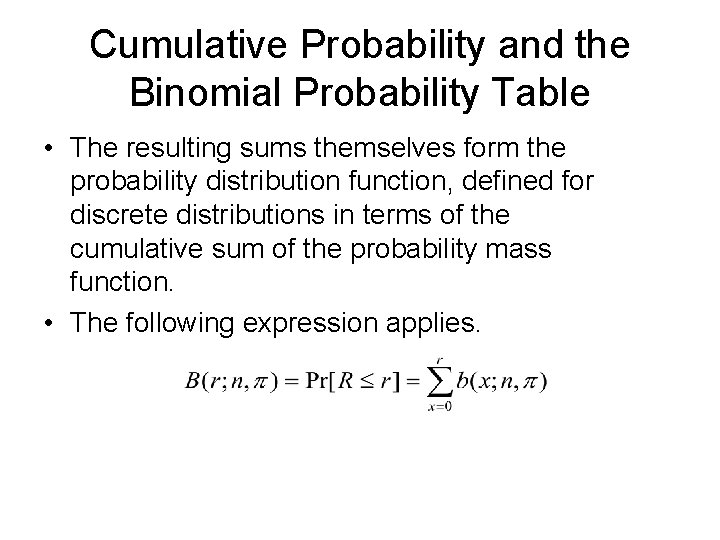
Cumulative Probability and the Binomial Probability Table • The resulting sums themselves form the probability distribution function, defined for discrete distributions in terms of the cumulative sum of the probability mass function. • The following expression applies.

See page 211, 212 and 214 for examples

The Normal Distribution • Most frequently encountered in statistics is the normal distribution, often referred to as the Gaussian distribution. • Every normal frequency curve is centered on the population mean and symmetric about this point

NORMAL DISTRIBUTION • The probability density function – f(x), area and the effect of changing mean and variances • Given x, find probability • Given probability, find x

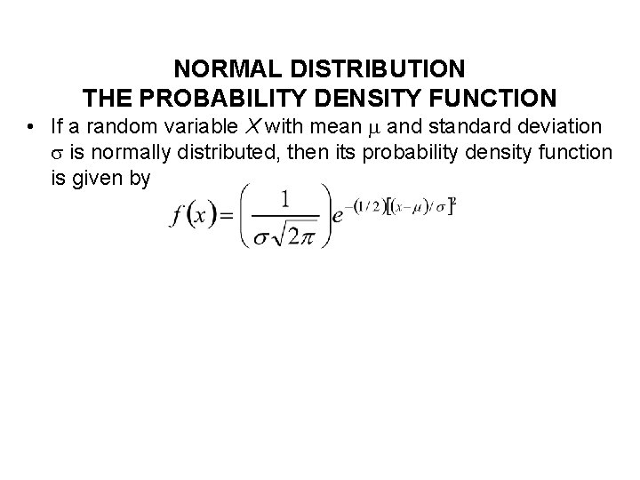
NORMAL DISTRIBUTION THE PROBABILITY DENSITY FUNCTION • If a random variable X with mean and standard deviation is normally distributed, then its probability density function is given by

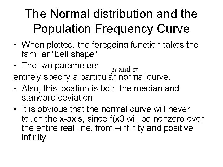
The Normal distribution and the Population Frequency Curve • When plotted, the foregoing function takes the familiar “bell shape”. • The two parameters entirely specify a particular normal curve. • Also, this location is both the median and standard deviation • It is obvious that the normal curve will never touch the x-axis, since f(x 0 will be nonzero over the entire real line, from –infinity and positive infinity.

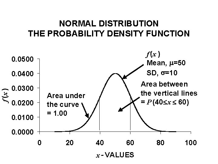
NORMAL DISTRIBUTION THE PROBABILITY DENSITY FUNCTION f (x ) Mean, =50 SD, =10 0. 0500 f (x ) 0. 0400 0. 0300 Area between the vertical lines = P (40 x 60) Area under the curve = 1. 00 0. 0200 0. 0100 0. 0000 0 20 40 60 x - VALUES 80 100

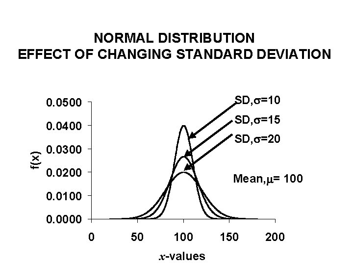
NORMAL DISTRIBUTION EFFECT OF CHANGING STANDARD DEVIATION SD, =10 0. 0500 SD, =15 f(x) 0. 0400 SD, =20 0. 0300 0. 0200 Mean, = 100 0. 0000 0 50 100 x-values 150 200

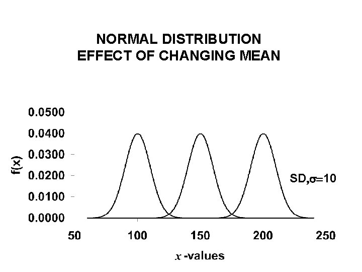
NORMAL DISTRIBUTION EFFECT OF CHANGING MEAN SD, =10

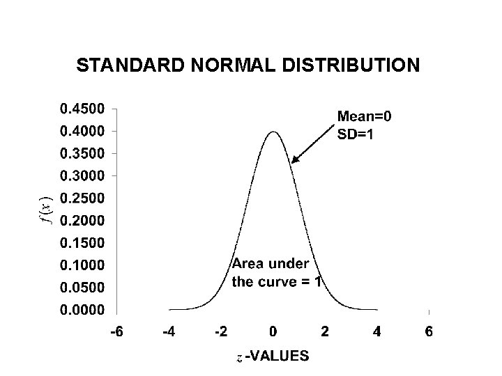
STANDARD NORMAL DISTRIBUTION

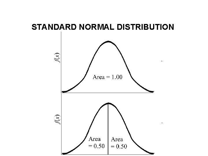
STANDARD NORMAL DISTRIBUTION

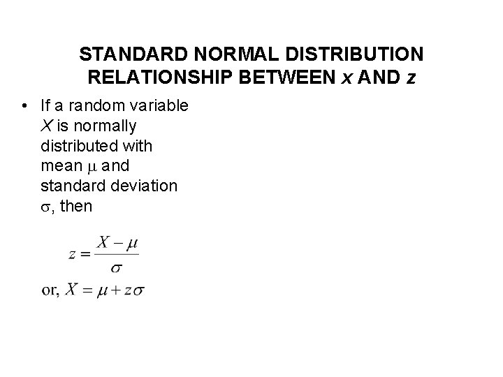
STANDARD NORMAL DISTRIBUTION RELATIONSHIP BETWEEN x AND z • If a random variable X is normally distributed with mean and standard deviation , then

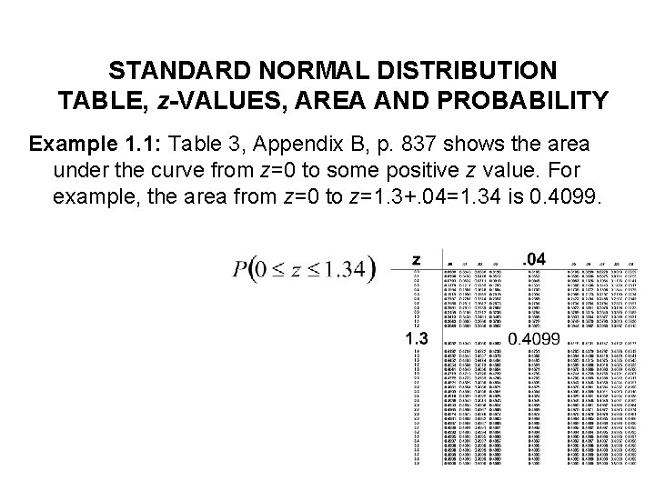
STANDARD NORMAL DISTRIBUTION TABLE, z-VALUES, AREA AND PROBABILITY Example 1. 1: Table 3, Appendix B, p. 837 shows the area under the curve from z=0 to some positive z value. For example, the area from z=0 to z=1. 3+. 04=1. 34 is 0. 4099.