Binocular Stereo 1 Topics 1 Principle 2 binocular

Binocular Stereo #1

Topics 1. Principle 2. binocular stereo basic equation 3. epipolar line 4. features and strategies for matching

Binocular stereo single image is ambiguous A a’ a” another image taken from a different direction gives the unique 3 D point

Epipolar line constraints Epipolar line One image point Possible line of sight Base line Epipolar plane Corresponding points lie on the Epipolar lines Epipolar line constratints
 C 1 e 2 Epipoles: • intersections of baseline with")
Epipolar geometry (multiple points) C 1 e 2 Epipoles: • intersections of baseline with image planes • projection of the optical center in another image • the vanishing points of camera motion direction C 2

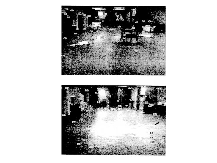
Examples of epipolar geometry

Examples of epipolar geometry

Examples of epipolar geometry

Characteristics of epipolar line • rectification

Basic binocular stereo equation A physical point left image point right image plane left image center focal length right image center z World coordinate system base line length

Camera Model Pinhole camera
 View point (Optical center) y")
Camera Model geometry Y Perspective projection X (x, y) View point (Optical center) y x (X, Y, Z) (s. X, s. Y, s. Z) f : focal length -Z Image plane
 x”-x’:")
Basic binocular stereo equation d+x d-x -z x’ x” d d z=-2 df/(x”-x’) x”-x’: disparity 2 d : base line length z f

Classic algorithms for binocular Stereo Marr-Poggio-Grimson Nishihara-Poggio Lucas-Kanade Ohta-Kanade Matthie-Kanade Okutomi-Kanade Baker Hannah Moravec Barnard-Thompson MIT group CMU group Stanford group

Features for matching a. brightness b. edges c. edge intervals d. interest points 10 11 12 11 15 16

Strategies for matching a. relaxation 10 10 5 10 10 10 10 10 b. coarse to fine c. dynamic programming global optimam local optimam

Main purpose of development Marr-Poggio-Grimson Nishihara-Poggio simulate human stereo Lucas-Kanade Ohta-Kanade Matthie-Kanade Okutomi-Kanade map making Baker Hannah Moravec map making navigation Barnard-Thompson navigation
 edges intervals Lucas-Kanade Ohta-Kanade Matthie-Kanade Okutomi-Kanade brightness(gradient)")
Features for matching Marr-Poggio-Grimson Nishihara-Poggio points(random dots) edges intervals Lucas-Kanade Ohta-Kanade Matthie-Kanade Okutomi-Kanade brightness(gradient) intervals brightness Baker Hannah Moravec edges interest points Barnard-Thompson interest points

Strategies for matching Marr-Poggio-Grimson Nishihara-Poggio relaxation coarse to fine Lucas-Kanade Ohta-Kanade Matthie-Kanade Okutomi-Kanade relaxation dynamic programming Relaxation (Kalman filter) relaxation Baker Hannah Moravec dynamic programming coarse to fine Barnard-Thompson relaxation

Summary 1. binocular stereo takes two images of 3 D point from two different positions and determines its 3 D coordinate system. 2. Epipolar line 2 D matching ↓ 1 D matching 3. Features for matching ---brightness, edge interval, interest point 4. Strategies for matching ---relaxation, coarse to fine, dynamic programming 5. Read B&B pp. 88 -93 Horn pp. 299 -303

Binocular Stereo #2

Topics case study area-based stereo Marr-poggio stereo simulate human visual system Ohta-Kanade stereo aerial image analysis Moravec stereo navigation

Classification of stereo method 1. Features for matching a. brightness value b. point c. edge d. region 2. Strategies for matching a. brute-force (not a strategy ? ? ? ) b. coarse-to-fine c. relaxation d. dynamic programming 3. Constraints for matching a. epipolar lines b. disparity limit c. continuity d. uniqueness

Area-based stereo 1. method b c 2. problem a. trade-off of window size and resolution b. dull peak b c

Area-based stereo 1. Features for matching a. brightness value b. point c. edge d. region 2. Strategies for matching a. brute-force (not a strategy ? ? ? ) b. coarse-to-fine c. relaxation d. dynamic programming 3. Constraints for matching a. epipolar lines b. disparity limit c. continuity d. uniqueness
 Simulating human visual system (random dot stereo gram) Marr, Poggio “Coopertive computation")
Marr-Poggio Stereo(`76) Simulating human visual system (random dot stereo gram) Marr, Poggio “Coopertive computation of stereo disparity” Science 194, 283 -287

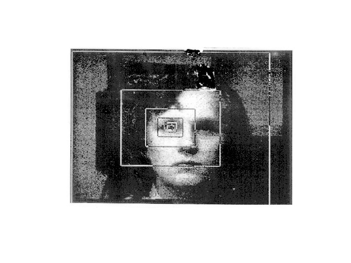
Input : random dot stereo left image random dot shift the catch pat right image we can see the height different between the central and peripheral area

Constraints – Epipolar line constraint – Uniqueness constraint » each point in a image has only one depth value O. K. No. – Continuity constraint » each point is almost sure to have a depth value near the values of neighbors O. K. No.

D E F A A B C B D C E F Uniqueness constraint prohibits two or more matching points on one horizontal or vertical lines (E-A) A (E-B) B prohibit C (E-C) continuity constraint attracts more matching on a diagonal line (D-A) attract (E-B) (F-C) Same depth

relaxation 10 10 5 10 10 10 10 10 n+1
 1. Features for matching a. brightness value b. point c. edge d.")
Marr-Poggio Stereo(`76) 1. Features for matching a. brightness value b. point c. edge d. region 2. Strategies for matching a. brute-force (not a strategy ? ? ? ) b. coarse-to-fine c. relaxation d. dynamic programming 3. Constraints for matching a. epipolar lines b. disparity limit c. continuity d. uniqueness simulate the human visual system (MIT)
 Map making Ohta, Kanade “Stereo by intra- and inter-scanline search using dynamic")
Ohta-Kanade Stereo(`85) Map making Ohta, Kanade “Stereo by intra- and inter-scanline search using dynamic programming” , IEEE Trans. , Vol. PAMI-7, No. 2, pp. 139 -14

now matching become 1 D to 1 D L 1 L 2 L 3 L 4 L 5 L 6 R 1 R 2 R 3 R 4 R 5 R 6 L disparity R yet, N line * ML * MR (512 * 100 * 10 m sec = 15 hours)

Path Search u Matching problem can be considered as a path search problem u define a cost at each candidate of path segment based some ad-hoc function 10 100

Dynamic programming We can formalize the path finding problem as the following iterative formula optimum cost to K 3 0 2 1 cost between M and K Optimum costs are known

stereo pair edges

path disparity depth

stereo pair edges depth
 1. Features for matching a. brightness value b. point Brightness of interval")
Ohta-Kanade Stereo(`85) 1. Features for matching a. brightness value b. point Brightness of interval c. edge d. region 2. Strategies for matching a. brute-force (not a strategy ? ? ? ) b. coarse-to-fine c. relaxation d. dynamic programming 3. Constraints for matching a. epipolar lines b. disparity limit c. continuity d. uniqueness aerial image analysis (CMU)
 navigation Moravec “Visual mapping by a robot rover” Proc 6 th IJCAI,")
Moravec Stereo(`79) navigation Moravec “Visual mapping by a robot rover” Proc 6 th IJCAI, pp. 598 -600 (1979)

Moravec’s cart Slide stereo Motion stereo
 u = 36 stereo pairs!!! each stereo has an")
Slider stereo (9 eyes stereo) u = 36 stereo pairs!!! each stereo has an uncertainty measure uncertainty = 1 / base-line u each stereo has a confidence measure u u 9 C 2 long base line large uncertainty

Coarse to fine matching expand matching

area: confidence measure σ estimated distance σ: uncertainty measure 9 C 2 = 36 curves Interest point
 1. Features for matching a. brightness value b. point c. edge interest")
Moravec Stereo(`81) 1. Features for matching a. brightness value b. point c. edge interest point d. region 2. Strategies for matching a. brute-force (not a strategy ? ? ? ) b. coarse-to-fine c. relaxation d. dynamic programming 3. Constraints for matching a. epipolar lines b. disparity limit c. continuity d. uniqueness navigation (Stanford)

Summary 1. Two images from two different positions give depth information 2. Epipolar line and plane 3. Basic equation Z=-2 df/(x”-x’) x”-x’: disparity 2 d : base line length 4. case study area-based stereo Marr-poggio stereo simulate human visual system Ohta-Kanade stereo aerial image analysis Moravec stereo navigation 5. Read Horn pp. 299 -303

F matrix

Camera Model Pinhole camera
 View point (Optical center) y")
Camera Model geometry Y Perspective projection X (x, y) View point (Optical center) y x (X, Y, Z) (s. X, s. Y, s. Z) f : focal length -Z Image plane
 (Linear)")
Camera Model Perspective projection formularization Projection matrix Perspective projection Affine projection (Non-linear) (Linear)

Affine Camera Models General formularization • Orthographic • Perspective • Affine camera

Affine Cameras perspective orthographic Focal length Distance from camera

Intrinsic parameters CCD elements CCD : an actual picture Not equal ! Image plane : an ideal image
 v")
Intrinsic parameters An ideal image on the Image plane y v (x, y) v 0 x θ An actual picture u 0 u (u, v)
")
Intrinsic parameters e. g. perspective projection Intrinsic matrix Projection matrix (normalized)

Extrinsic parameters Z Y X

Extrinsic parameters Z Y X

Extrinsic parameters

Extrinsic parameters R : rotation matrix t : translation vector
 (X, Y, Z) Z picture (u, v) Y R,")
Summary (intrinsic & extrinsic parameters) (X, Y, Z) Z picture (u, v) Y R, t World coordinate Camera coordinate X World coordinate
 (X, Y, Z) Z picture (u, v) Y R,")
Summary (intrinsic & extrinsic parameters) (X, Y, Z) Z picture (u, v) Y R, t World coordinate X 3 × 4 matrix

Epipolar geometry Essential matrix : E C 2 C 1 R
 Image 1 Image 2 Pictures (actual) Fundamental")
Essential & Fundamental matrix Image planes (ideal) Image 1 Image 2 Pictures (actual) Fundamental matrix : F
 (u’, v’, 1) F &")
F matrix picture 1 picture 2 (u, v, 1) (u’, v’, 1) F & (u, v) known Calculate the epipolar line
")
Computing F matrix (Linear solution)

Corner detector x Extract interest points in each images y Harris corner detector

Matching or
 Suppose we found 8 pairs of corresponding points ·····")
Computing F matrix (Linear solution) Suppose we found 8 pairs of corresponding points ·····
 Epipolar pencil by linear solution (due to noise and")
Computing F matrix (Singularity constraint) Epipolar pencil by linear solution (due to noise and error)
 Singular value decomposition (SVD) Without noise, σ3 must be")
Computing F matrix (Singularity constraint) Singular value decomposition (SVD) Without noise, σ3 must be 0 modification
")
Computing F matrix (Singularity constraint)

Summary u Pinhole camera and Affine camera u Intrinsic and extrinsic camera parameter u Epipolar geometry u Fundamental matrix
- Slides: 74