Binary Thresholding Threshold detection Variations Mathematical Morphology Connectivity
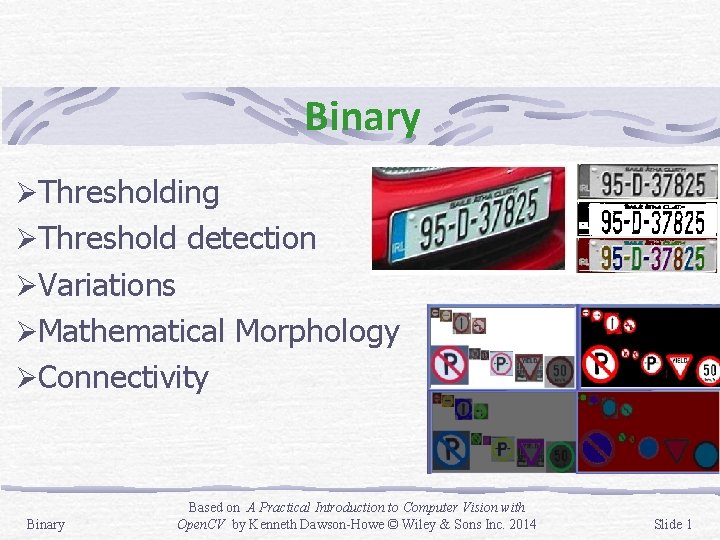
Binary ØThresholding ØThreshold detection ØVariations ØMathematical Morphology ØConnectivity Binary Based on A Practical Introduction to Computer Vision with Open. CV by Kenneth Dawson-Howe © Wiley & Sons Inc. 2014 Slide 1
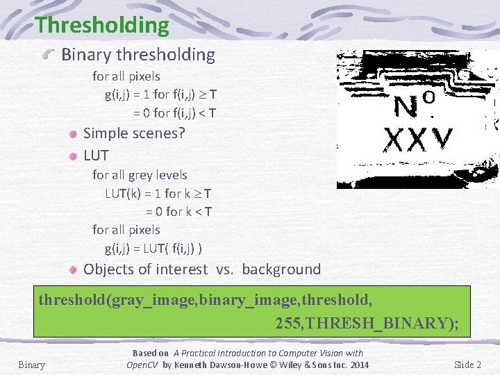
Thresholding Binary thresholding for all pixels g(i, j) = 1 for f(i, j) T = 0 for f(i, j) < T Simple scenes? LUT for all grey levels LUT(k) = 1 for k T = 0 for k < T for all pixels g(i, j) = LUT( f(i, j) ) Objects of interest vs. background threshold(gray_image, binary_image, threshold, 255, THRESH_BINARY); Binary Based on A Practical Introduction to Computer Vision with Open. CV by Kenneth Dawson-Howe © Wiley & Sons Inc. 2014 Slide 2
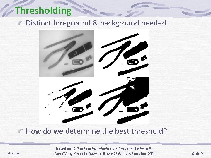
Thresholding Distinct foreground & background needed How do we determine the best threshold? Binary Based on A Practical Introduction to Computer Vision with Open. CV by Kenneth Dawson-Howe © Wiley & Sons Inc. 2014 Slide 3
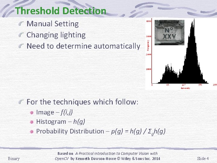
Threshold Detection Manual Setting Changing lighting Need to determine automatically For the techniques which follow: Image – f(i, j) Histogram – h(g) Probability Distribution – p(g) = h(g) / Σgh(g) Binary Based on A Practical Introduction to Computer Vision with Open. CV by Kenneth Dawson-Howe © Wiley & Sons Inc. 2014 Slide 4
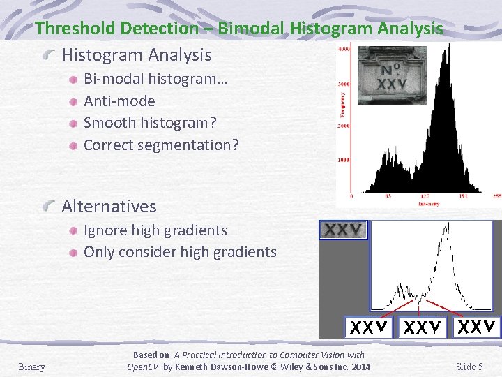
Threshold Detection – Bimodal Histogram Analysis Bi-modal histogram… Anti-mode Smooth histogram? Correct segmentation? Alternatives Ignore high gradients Only consider high gradients Binary Based on A Practical Introduction to Computer Vision with Open. CV by Kenneth Dawson-Howe © Wiley & Sons Inc. 2014 Slide 5
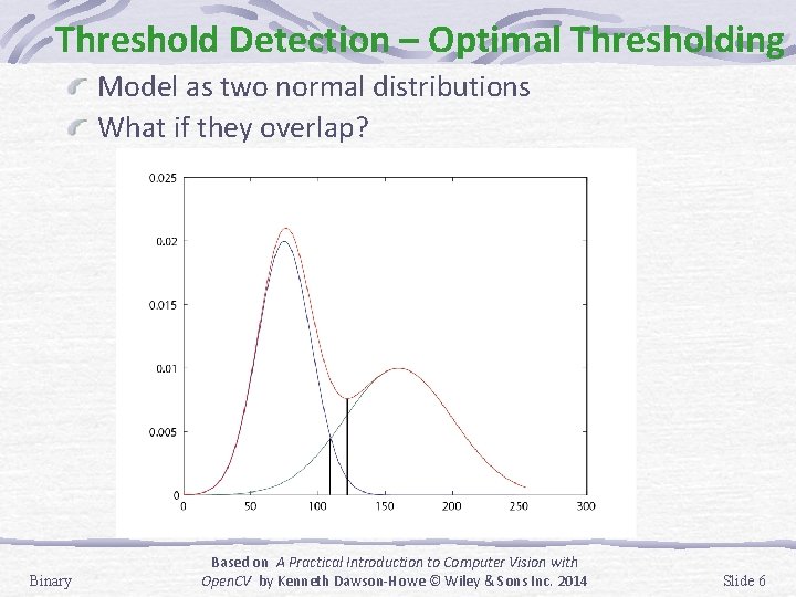
Threshold Detection – Optimal Thresholding Model as two normal distributions What if they overlap? Binary Based on A Practical Introduction to Computer Vision with Open. CV by Kenneth Dawson-Howe © Wiley & Sons Inc. 2014 Slide 6
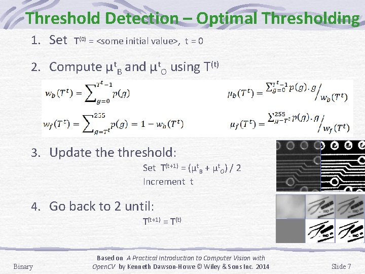
Threshold Detection – Optimal Thresholding 1. Set T(0) = <some initial value>, t = 0 2. Compute µt. B and µt. O using T(t) 3. Update threshold: Set T(t+1) = (µt. B + µt. O) / 2 Increment t 4. Go back to 2 until: T(t+1) = T(t) Binary Based on A Practical Introduction to Computer Vision with Open. CV by Kenneth Dawson-Howe © Wiley & Sons Inc. 2014 Slide 7
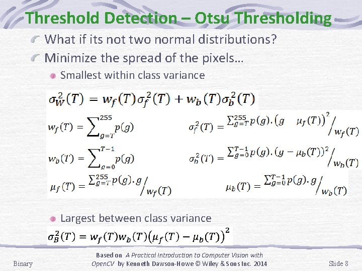
Threshold Detection – Otsu Thresholding What if its not two normal distributions? Minimize the spread of the pixels… Smallest within class variance Largest between class variance Binary Based on A Practical Introduction to Computer Vision with Open. CV by Kenneth Dawson-Howe © Wiley & Sons Inc. 2014 Slide 8

Threshold Detection – Otsu Thresholding threshold( gray_image, binary_image, threshold, 255, THRESH_BINARY | THRESH_OTSU ); Binary Based on A Practical Introduction to Computer Vision with Open. CV by Kenneth Dawson-Howe © Wiley & Sons Inc. 2014 Slide 9
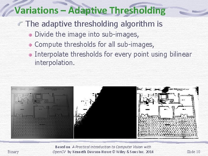
Variations – Adaptive Thresholding The adaptive thresholding algorithm is Divide the image into sub-images, Compute thresholds for all sub-images, Interpolate thresholds for every point using bilinear interpolation. Binary Based on A Practical Introduction to Computer Vision with Open. CV by Kenneth Dawson-Howe © Wiley & Sons Inc. 2014 Slide 10
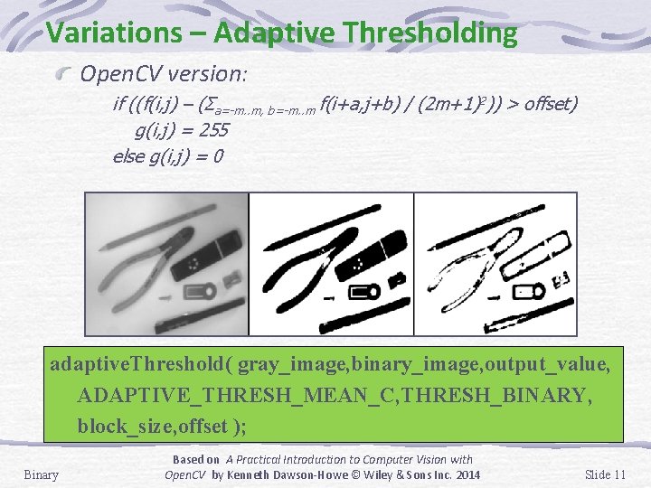
Variations – Adaptive Thresholding Open. CV version: if ((f(i, j) – (Σa=-m. . m, b=-m. . m f(i+a, j+b) / (2 m+1)2)) > offset) g(i, j) = 255 else g(i, j) = 0 adaptive. Threshold( gray_image, binary_image, output_value, ADAPTIVE_THRESH_MEAN_C, THRESH_BINARY, block_size, offset ); Binary Based on A Practical Introduction to Computer Vision with Open. CV by Kenneth Dawson-Howe © Wiley & Sons Inc. 2014 Slide 11
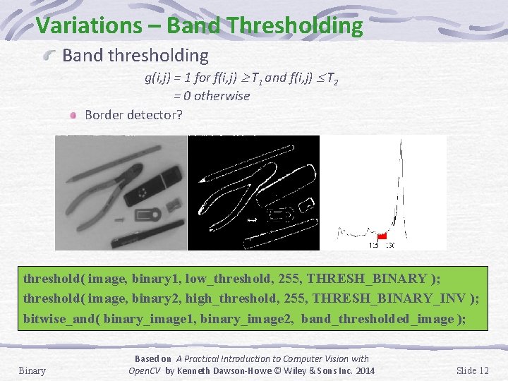
Variations – Band Thresholding Band thresholding g(i, j) = 1 for f(i, j) T 1 and f(i, j) T 2 = 0 otherwise Border detector? threshold( image, binary 1, low_threshold, 255, THRESH_BINARY ); threshold( image, binary 2, high_threshold, 255, THRESH_BINARY_INV ); bitwise_and( binary_image 1, binary_image 2, band_thresholded_image ); Binary Based on A Practical Introduction to Computer Vision with Open. CV by Kenneth Dawson-Howe © Wiley & Sons Inc. 2014 Slide 12
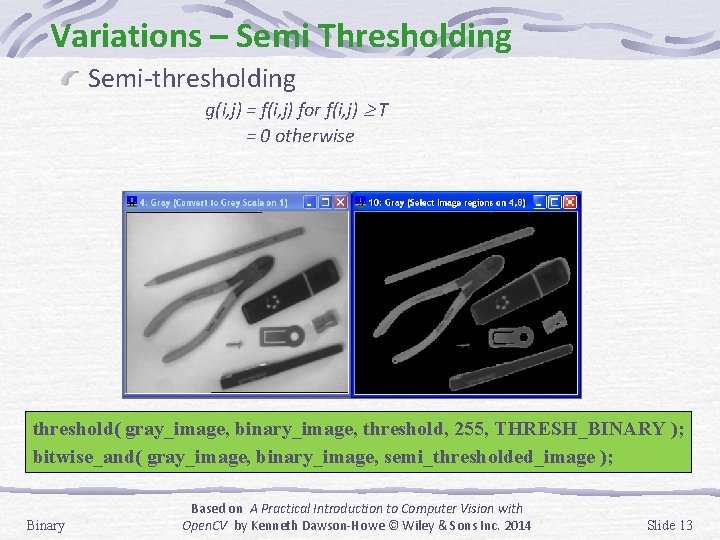
Variations – Semi Thresholding Semi-thresholding g(i, j) = f(i, j) for f(i, j) T = 0 otherwise threshold( gray_image, binary_image, threshold, 255, THRESH_BINARY ); bitwise_and( gray_image, binary_image, semi_thresholded_image ); Binary Based on A Practical Introduction to Computer Vision with Open. CV by Kenneth Dawson-Howe © Wiley & Sons Inc. 2014 Slide 13
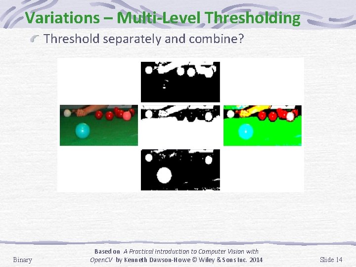
Variations – Multi-Level Thresholding Threshold separately and combine? Binary Based on A Practical Introduction to Computer Vision with Open. CV by Kenneth Dawson-Howe © Wiley & Sons Inc. 2014 Slide 14
Mathematical Morphology – Introduction Based on algebra of non-linear operators operating on object shape Performs many tasks better and more quickly than standard approaches Separate part of image analysis Operates with points sets, their connectivity and shape Main uses: Pre-processing Object structure enhancement Segmentation Description of objects Binary Based on A Practical Introduction to Computer Vision with Open. CV by Kenneth Dawson-Howe © Wiley & Sons Inc. 2014 Slide 15
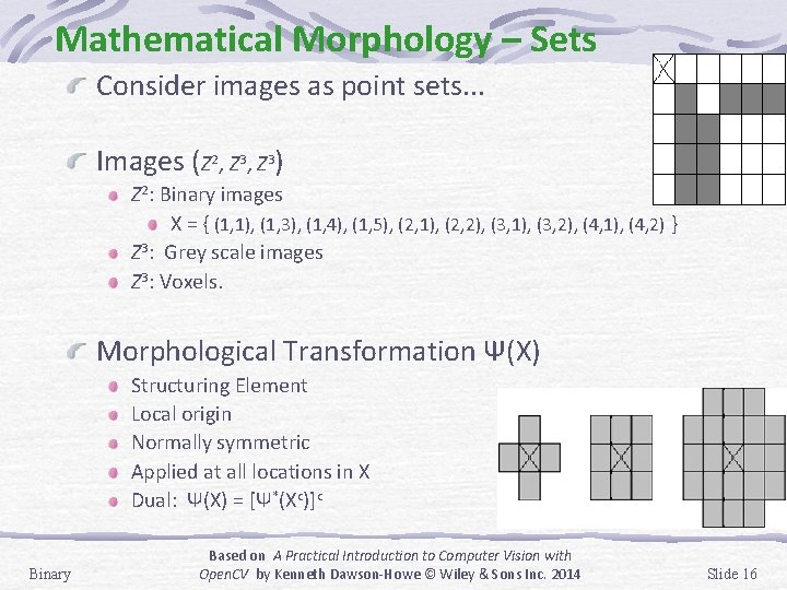
Mathematical Morphology – Sets Consider images as point sets. . . Images (Z 2, Z 3) Z 2: Binary images X = { (1, 1), (1, 3), (1, 4), (1, 5), (2, 1), (2, 2), (3, 1), (3, 2), (4, 1), (4, 2) } Z 3: Grey scale images Z 3: Voxels. Morphological Transformation Ψ(X) Structuring Element Local origin Normally symmetric Applied at all locations in X Dual: Ψ(X) = [Ψ*(Xc)]c Binary Based on A Practical Introduction to Computer Vision with Open. CV by Kenneth Dawson-Howe © Wiley & Sons Inc. 2014 Slide 16
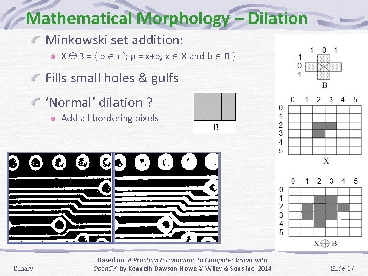
Mathematical Morphology – Dilation Minkowski set addition: X B = { p ε 2; p = x+b, x X and b B } Fills small holes & gulfs ‘Normal’ dilation ? Add all bordering pixels Binary Based on A Practical Introduction to Computer Vision with Open. CV by Kenneth Dawson-Howe © Wiley & Sons Inc. 2014 Slide 17
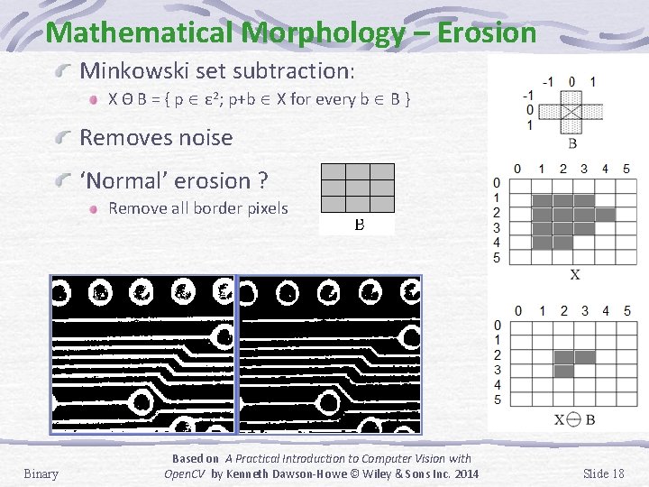
Mathematical Morphology – Erosion Minkowski set subtraction: X Θ B = { p ε 2; p+b X for every b B } Removes noise ‘Normal’ erosion ? Remove all border pixels Binary Based on A Practical Introduction to Computer Vision with Open. CV by Kenneth Dawson-Howe © Wiley & Sons Inc. 2014 Slide 18
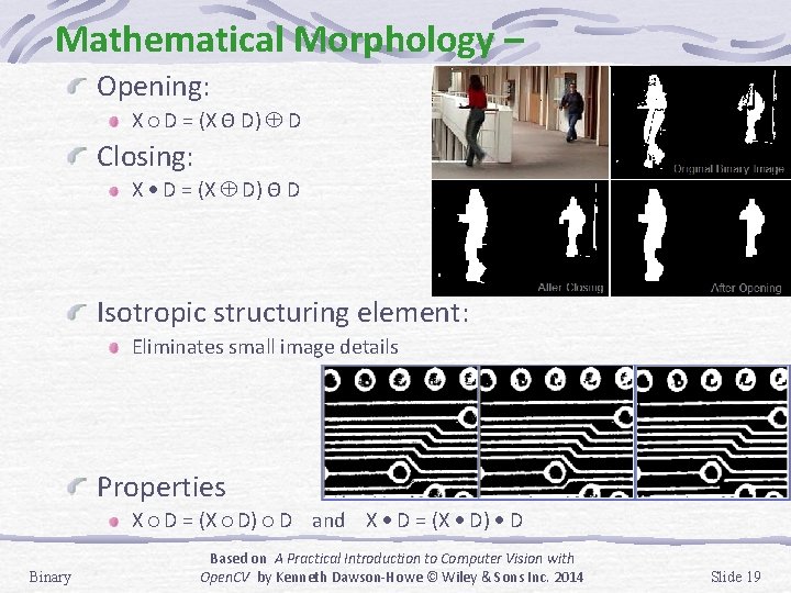
Mathematical Morphology – Opening: X D = (X Θ D) D Closing: X D = (X D) Θ D Isotropic structuring element: Eliminates small image details Properties X D = (X D) D and X D = (X D) D Binary Based on A Practical Introduction to Computer Vision with Open. CV by Kenneth Dawson-Howe © Wiley & Sons Inc. 2014 Slide 19
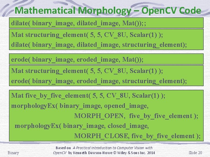
Mathematical Morphology – Open. CV Code dilate( binary_image, dilated_image, Mat()); ; Mat structuring_element( 5, 5, CV_8 U, Scalar(1) ); dilate( binary_image, dilated_image, structuring_element); erode( binary_image, eroded_image, Mat()); Mat structuring_element( 5, 5, CV_8 U, Scalar(1) ); erode( binary_image, eroded_image, structuring_element); Mat five_by_five_element( 5, 5, CV_8 U, Scalar(1) ); morphology. Ex( binary_image, opened_image, MORPH_OPEN, five_by_five_element ); morphology. Ex( binary_image, closed_image, MORPH_CLOSE, five_by_five_element ); Binary Based on A Practical Introduction to Computer Vision with Open. CV by Kenneth Dawson-Howe © Wiley & Sons Inc. 2014 Slide 20
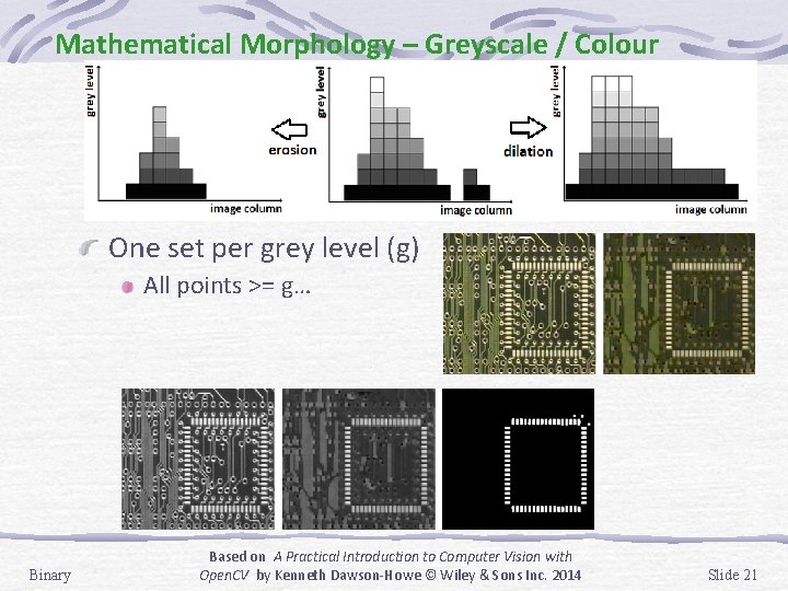
Mathematical Morphology – Greyscale / Colour One set per grey level (g) All points >= g… Binary Based on A Practical Introduction to Computer Vision with Open. CV by Kenneth Dawson-Howe © Wiley & Sons Inc. 2014 Slide 21
Mathematical Morphology – Local maxima Can be used to locate local maxima and minima Mat dilated, thresholded_input, local_maxima, thresholded_8 bit; dilate( input, dilated, Mat()); compare( input, dilated, local_maxima, CMP_EQ ); threshold( input, thresholded_input, threshold, 255, THRESH_BINARY ); thresholded_input. convert. To( thresholded_8 bit, CV_8 U ); bitwise_and( local_maxima, thresholded_8 bit, local_maxima ); Binary Based on A Practical Introduction to Computer Vision with Open. CV by Kenneth Dawson-Howe © Wiley & Sons Inc. 2014 Slide 22
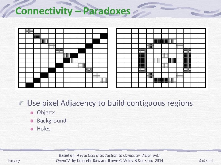
Connectivity – Paradoxes Use pixel Adjacency to build contiguous regions Objects Background Holes Binary Based on A Practical Introduction to Computer Vision with Open. CV by Kenneth Dawson-Howe © Wiley & Sons Inc. 2014 Slide 23

Connectivity – 4 adjacency & 8 adjacency Have to use either 4 -adjacency or 8 -adjacency Label each non-zero pixel… Binary Based on A Practical Introduction to Computer Vision with Open. CV by Kenneth Dawson-Howe © Wiley & Sons Inc. 2014 Slide 24
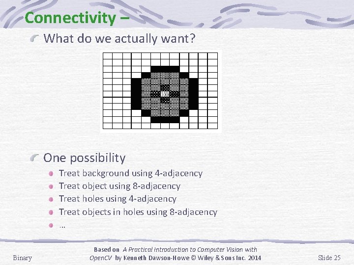
Connectivity – What do we actually want? One possibility Treat background using 4 -adjacency Treat object using 8 -adjacency Treat holes using 4 -adjacency Treat objects in holes using 8 -adjacency … Binary Based on A Practical Introduction to Computer Vision with Open. CV by Kenneth Dawson-Howe © Wiley & Sons Inc. 2014 Slide 25
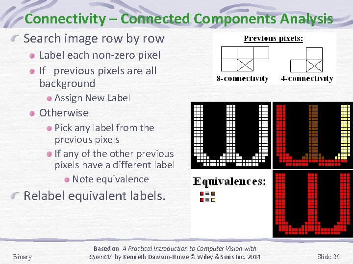
Connectivity – Connected Components Analysis Search image row by row Label each non-zero pixel If previous pixels are all background Assign New Label Otherwise Pick any label from the previous pixels If any of the other previous pixels have a different label Note equivalence Relabel equivalent labels. Binary Based on A Practical Introduction to Computer Vision with Open. CV by Kenneth Dawson-Howe © Wiley & Sons Inc. 2014 Slide 26
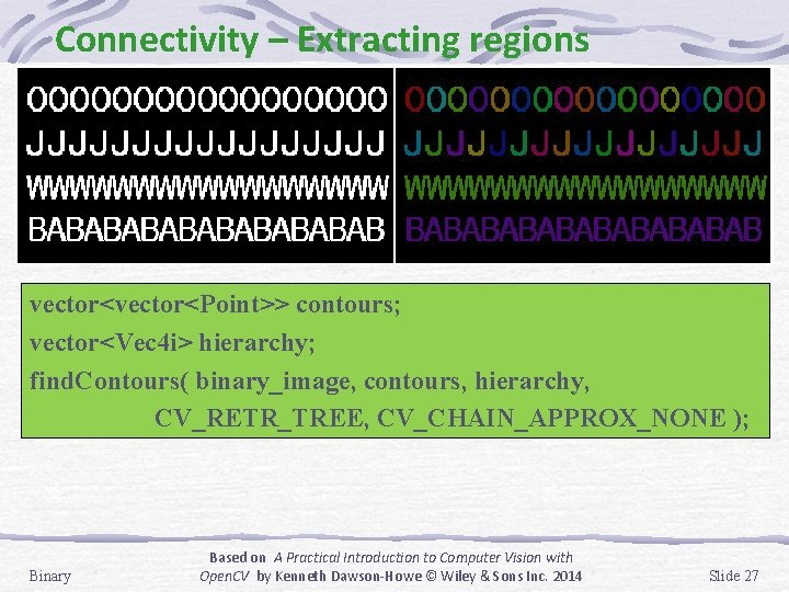
Connectivity – Extracting regions vector<Point>> contours; vector<Vec 4 i> hierarchy; find. Contours( binary_image, contours, hierarchy, CV_RETR_TREE, CV_CHAIN_APPROX_NONE ); Binary Based on A Practical Introduction to Computer Vision with Open. CV by Kenneth Dawson-Howe © Wiley & Sons Inc. 2014 Slide 27
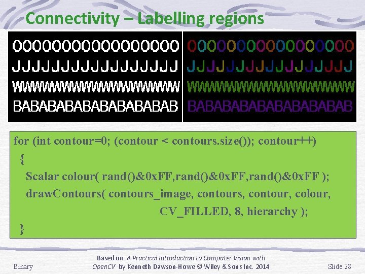
Connectivity – Labelling regions for (int contour=0; (contour < contours. size()); contour++) { Scalar colour( rand()&0 x. FF, rand()&0 x. FF ); draw. Contours( contours_image, contours, contour, colour, CV_FILLED, 8, hierarchy ); } Binary Based on A Practical Introduction to Computer Vision with Open. CV by Kenneth Dawson-Howe © Wiley & Sons Inc. 2014 Slide 28
- Slides: 28