Binary Thinning Algorithms Thick images Thin images Color

Binary Thinning Algorithms Thick images Thin images Color images Character Recognition (OCR)

5 basic structuring elements

Thinning of thick binary images Thinning: from many pixels width to just one • Much work has been done on the thinning of ``thick'' binary images, • where attempts are made to reduce shape outlines which are many pixels thick to outlines which are only one pixel thick. • Skeletonization

Thinning using Zhang and Suen is slightly algorithm [1984]. ) (b) increased Point just removed 8 7 image 26 25 results of the first pass results of the second pass final results

Example of Thinning algorithm from Zhang and Suen 1984

Example 1 of Rules for Thinning Algorithm Rule 1 Old one Rule 1 Don’t care Rule 2 All four rules can be illustrated like that New and old one Rule 3 Rule 4

Applying thinning to fault detection in PCB All lines are thinned to one pixel width Now you can check connectivity

Thinning Algorithm image Correct background shows desired shape of letter T • Thinning algorithm is sensitive to corrupted image segments Noise leads to lack of connectivity. BAD

Thinning applied after Edge Detection

Thinning of thin binary images Rules of binary thinning • We will present the rules used for the ``binary thinning'' which is applied to the edge images (found using the edge detector). • The rules are simple and quick to carry out, requiring only one pass through the image.

The SUSAN Thinning Algorithm

The SUSAN Thinning Algorithm • It follows a few simple rules – remove spurious or unwanted edge points – • add in edge points where they should be reported but have not been. The rules fall into three categories; – removing spurious or unwanted edge points – adding new edge points – shifting edge points to new positions. • Note that the new edge points will only be created if the edge response allows this. These all can be called “local improving” rules

The SUSAN Thinning Algorithm • The rules are listed according to the number of edge point neighbours which an edge point has (in the eight pixel neighbourhood) Discuss size of window and direction of movement 0 neighbors 1 neighbor 2 neighbors 3 neighbors

The SUSAN Thinning Algorithm • 0 neighbors. – Remove the edge point. • 1 neighbor. – Search for the neighbor with the maximum (non-zero) edge response, to continue the edge, and to fill in gaps in edges. • The responses used are those found by the initial stage of the SUSAN edge detector, before non-maximum suppression. • They are slightly weighted according to the existing edge orientation so that the edge will prefer to continue in a straight line. • An edge can be extended by a maximum of three pixels. Filling gaps by adding new edge points

The SUSAN Thinning Algorithm • 2 neighbours. “Edge response” is a measure of neighborhood – There are three possible cases: • 1. If the point is ``sticking out'' of an otherwise straight line, then compare its edge response to that of the corresponding point within the line. – If the potential point within the straight edge has an edge response greater than 0. 7 of the current point's response, move the current point into line with the edge. • 2. If the point is adjoining a diagonal edge then remove it. • 3. Otherwise, the point is a valid edge point. My point has two neighbors

The SUSAN Thinning Algorithm • More than 2 neighbours. – If the point is not a link between multiple edges then thin the edge. • This will involve a choice between the current point and one of its neighbours. • If this choice is made in a logical consistent way then a ``clean'' looking thinned edge will result.

The SUSAN Thinning Algorithm How rules are applied? • These rules are applied to every pixel in the image sequentially left to right and top to bottom. – If a change is made to the edge image then the current search point is moved backwards up to two pixels leftwards and upwards. – This means that iterative alterations to the image can be achieved using only one pass of the algorithm.

Thinning can remove certain types of lines from the image

Correct and Incorrect Thinning Examples • X correct • V misread as Y • 8 has noise added and not removed, wrong semantic network will be created

Good thinning examples • Here every symbol correctly thinned

Another set of. Thinning Rules for Thinning Rules Algorithm • Examples of rules for shifting up and down algorithm Down rules Up rules Old and new

Tracing Direction Tracing direction from left to right • Notation for points in window • Rules based on point replacements

Tracing Direction This pixed changed to white

Example of bad thinning • We would like to have one pixel width everywhere

Thinning algorithm for images from polygons

Typical errors of thinning algorithms

Gradient based thinning

Encoding shapes after thinning

Encoding to discrete angles • Image after thinning

Use of angles in encoding

Replacement of blocks with points Select the closest point Coding in 8 directions Also, coding in 4 directions or more directions

Polygon Approximation -Encoding • Two Methods are used: – Included objects – Minimal objects • Included objects We start with the set of rectangles with points inside Line Segments make minimum change to the line

• (a) original figure, (b) computation of distances, (c) connection of vertices, (d) resultant polygon start Method of minimal objects Draw straight angles

Encoding of figures • (a) completion of a figure • (b) partitioning to segments

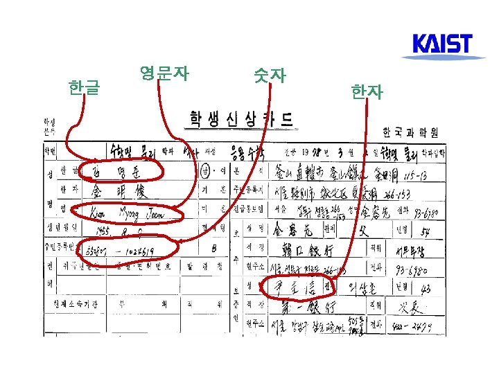
Examples of thinning: Processing Korean documents

KAIST

@99 Daru 김진형

Feature segmentation A Dist(A, B) vs Dist(A, C B C

Thinning Distortion at Crossing Point Overlapping Stroke @99 Daru 김진형

Thinning Erosion at end point Noise Sensitivity @99 Daru 김진형

Gray-scale Image @99 Daru 김진형

1: N Stroke Matching reference Model input character @99 Daru 김진형

Application: Figerprint Recognition

46

Fingerprint verification system

Same Fingerprints

Same Fingeprints? ?

Processing Whole Image • original

Binarization

Thinning: the essential

Still, what is a pattern?

Classification of signals • ECG

Classification in remote sensing

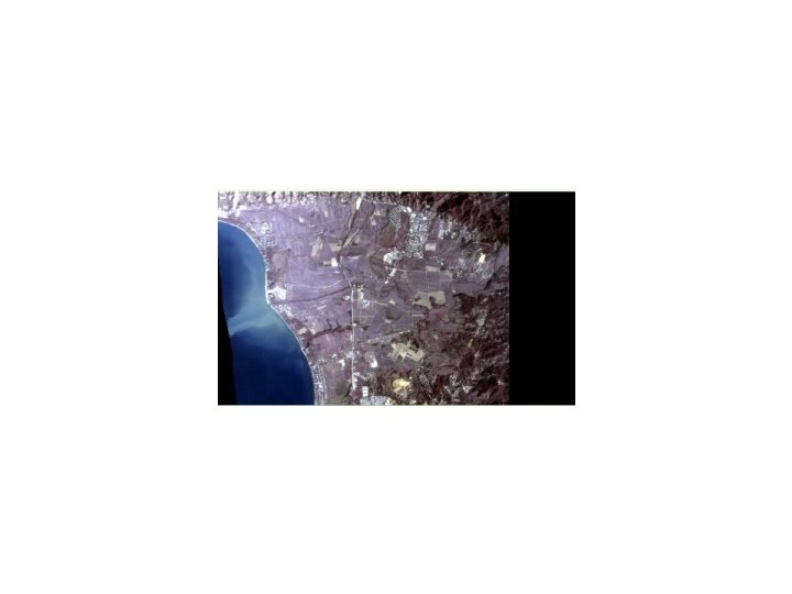
Classified Image

Pixel by Pixel Analysis

Histogram

Different Patterns: Corn (+) & Soybeans (*)

Optical Character Recognition

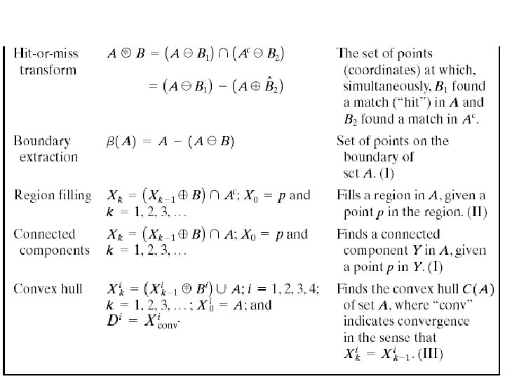
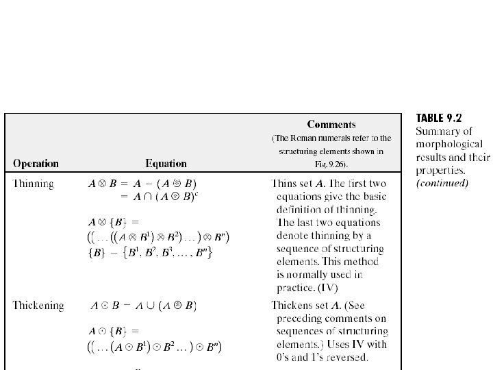
Thinning 63

Thickening 64

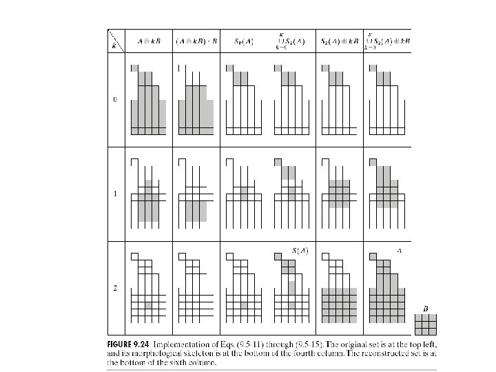
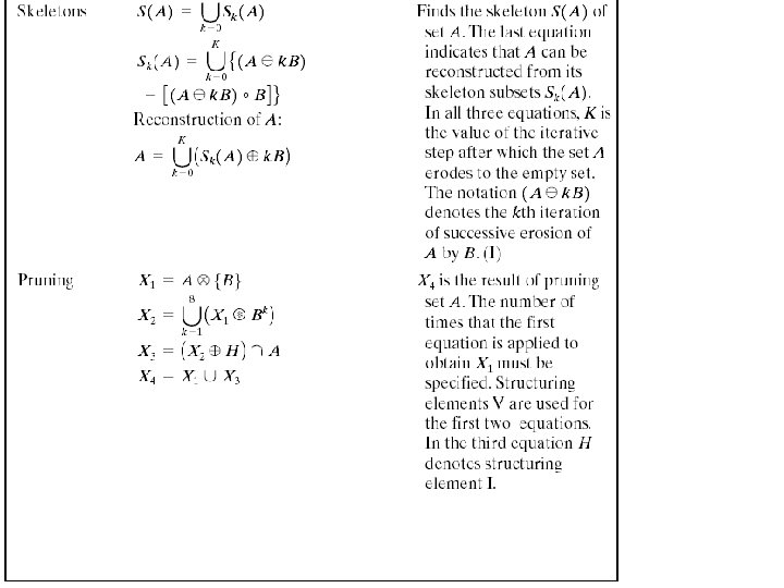
Skeletons

H = 3 x 3 structuring element of 1’s Pruning

Problems for students to solve • 1. Write a program for thinning with your own set of rules, that transform a kernel (3 by 3 or larger) to a point • 2. Write a program for thinning that replaces rectangle to rectangle according to one of sorted rules, about 10 rules. • 3. Compare with Zhang and Suen algorithm on images from FAB building interiors

More Problems to solve • The slides describe the rules used for the ``binary thinning'' which is applied to the edge images (found using the SUSAN edge detector - see [9, 8]) after non-maximum suppression has taken place. The rules are simple and quick to carry out, requiring only one pass through the image. Similar text originally appeared in Appendix B of [7]. • Write LISP program with the code of this edge detector and check it on similar images. • For examples and reviews of work on ``skeletonization'' see [6, 4, 1, 2, 5]. Implement any of these programs in LISP. Parametrize it.

Conclusion • Much work has been done on the thinning of ``thick'' binary images, where attempts are made to reduce shape outlines which are many pixels thick to outlines which are only one pixel thick. • However, because of the non-maximum suppression which is applied before thinning in edge detectors such as SUSAN, this kind of approach is not necessary.

Literature • 1 R. M. Haralick. Performance characterization in image analysis: Thinning, a case in point. Pattern Recognition Letters, 13: 5 --12, 1992. • 2 P. Kumar, D. Bhatnagar, and P. S. Umapathi Rao. Pseudo one pass thinning algorithm. Pattern Recognition Letters, 12: 543 --555, 1991. • 3 O. Monga, R. Deriche, G. Malandain, and J. P. Cocquerez. Recursive filtering and edge tracking: Two primary tools for 3 D edge detection. Image and Vision Computing, 9(4): 203 --214, 1991. • 4 J. A. Noble. Descriptions of Image Surfaces. D. Phil. thesis, Robotics Research Group, Department of Engineering Science, Oxford University, 1989. • 5 M. Otte and H. -H. Nagel. Extraction of line drawings from gray value images by non-local analysis of edge element structures. In Proc. 2 nd European Conf. on Computer Vision, pages 687 --695. Springer. Verlag, 1992.

Literature • 6 S. Pal. Some Low Level Image Segmentation Methods, Algorithms and their Analysis. Ph. D thesis, Indian Institute of Technology, 1991. • 7 S. M. Smith. Feature Based Image Sequence Understanding. D. Phil. thesis, Robotics Research Group, Department of Engineering Science, Oxford University, 1992. • 8 S. M. Smith. SUSAN -- a new approach to low level image processing. Internal Technical Report TR 95 SMS 1, Defence Research Agency, Chobham Lane, Chertsey, Surrey, UK, 1995. Available at www. fmrib. ox. ac. uk/~steve for downloading. • 9 S. M. Smith and J. M. Brady. SUSAN - a new approach to low level image processing. Int. Journal of Computer Vision, 23(1): 45 --78, May 1997.

SOURCES • Wanasanan Thongsongkrit • jkim@cs. kaist. ac. kr • Luis O. Jimenez-Rodriguez • • 傅楸善 & 王林農 0917533843 r 94922081@ntu. edu. tw 指導教授: 傅楸善博士