Binary Images Images only consist of two colors

Binary Images • Images only consist of two colors (tones): 0 0 0 0 white or black 0 0 0 0 0 255 255 255 255 0 0 0 0 0 • Image is characterized by location of white or black pixels Matrix Representation: 0 0 0 0 0 1 1 L={(3, 3), (3, 4), (4, 3), (4, 4)} Set Representation: Locations of white (or black) pixels

Binary Images 0 0 0 0 0 1 1

Binarization by Thresholding Original Histogram 50 Threshold = 50

Connectivity X’ Y Y’ X X and Y are connected X’ and Y’ are NOT connected Notation: if a and b are connected, we write a ≈ b

Pixel Neighborhoods and Connectivity Neighbors for discrete images 4 -neighbors • • 8 -neighbors A pixel is connected to its neighbors (w. same color) Reflexive: x ≈ x for all x Symmetric: if x ≈ y, then y ≈ x Transitive: if x ≈ y and y ≈ z, then x ≈ z

Why Rectangular Grid? • Hexagonal Grid – All identical neighbors – Non-recursive, Multi-resolution tricky • Triangular Grid – 3 types of neighbors • So we are left with the rectangular grid…

Connected Components • A separate definition for 4/8 neighborhoods. • A set of pixels S is a Connected Component if for each pixel pair (x 1, y 1) є S and (x 2, y 2) є S there is a path between them such that every two successive pixels in the path are in S and are Xneighbors. (X = 4, 8). 1 black 8 -component 3 black 4 -components

Objects and Backgrounds • 8 -neighborhood: – 1 black component – 1 white component • 4 -neighborhood: – 4 black components – 2 white components (background, hole) • Conflict! • Always choose different neighborhood metrics for objects and backgrounds

Computing Connected Components ? ? P=1 • Pass 1: Raster scan image: top → bottom, left → right – For every pixel P=1 (object), test top and left neighbors – If the 2 neighbors =0: assign a new mark to P – If 1 of the neighbors =1: assign the neighbor's mark to P – If both neighbors = 1: assign the left neighbor's mark to P, and note equivalence between marks of the 2 neighbors • Compute Equivalence Classes using Union-Find • Pass 2: Replace each mark with the number of it’s equivalence class

Connected Components – Example Original Binary image Pass 1: Pass 2:

Edges • C = A connected component of object A. • D = A connected component of Ā • The D-Edge of C = the set of all pixels in C that have a neighboring pixel in D. – neighboring-8 if C is 4 -connected – neighboring-4 if C is 8 -connected D E Object C D Edge of C E 4 Edge of C E 8 Edge of C

Chain Codes for Edges 1 1 2 0 7 6 6 6 2 3 4 -neighbor 8 -neighbor 2 4 3 0 6 2 3 5 Chain code of 4 -edge: 1 4 0 5 7 6 5 076666553321212 Can mark starting point

Invariance of chain code (Rot & Trans) 066444201066 067644222 Natural invariance to translation. Work needed for Rotation. Curvature = Differences in chain code values mod 8: 202002271202 271202002 Cyclic permutation which produces the smallest number: 002271202

Distances • Given 2 points P=(x, y), Q=(u, v) • Euclidean Distance • City Block Distance • Chessboard Distance • In Example: P=(1, 1); Q=(4, 8) • In General:

Distance Properties • Circle: all points having an equal distance d 8 2 2 2 1 1 1 2 2 1 0 1 2 2 1 1 1 2 2 2 d 4 2 2 2 1 2 1 0 1 2 2 • de, d 4, and d 8 are metrics de 0

Distance Maps / Transforms Distance from Set of Points (closest point). Black=0. Euclidean City Block Chessboard Distance from Boundary (closest boundary point)

2 -Paths Distance Transform • Given a set of pixels S, calculate the distance of other pixels to S. 4 8 P P dist • Raster scan image • Consider previously visited pixels (N 1 = green) • In reverse scan, consider (N 2 = blue)

Example Distance Transform measuring d 4: P 1 0 0 1 2 3 0 1 2 1 0 0 0 1 1 2 3 0 1 2 1 0 0 0 2 3 4 1 2 3 2 1 S is marked as 1 Pass 1: d’(P, S) Pass 2: d(P, S)

Skeleton-Medial Axis • A skeleton point is a local maximum (4 -8) in the distance transform 1 1 1 1 1 • Using 8 -neighborhood 1 2 2 2 2 1 2 3 3 3 2 • Using 4 -neighborhood 1 2 2 2 2 1 • – Centers of Maximal Disks That touch boundary in two points • Connectivity not preserved 1 1 1 1

Medial Axis - Grassfire • Suppose that a fire line propagates with constant speed from the contour of a connected object towards its inside, then all those points lying in positions where at least two wave fronts of the fire line meet during the propagation will constitute a form of a skeleton • Examples

Medial Axis Transform

Banana Peeling Skeleton • Iteratively check all 4 direction (D=W, N, E, S) • Remove a pixel from S if it is a border from direction D, and if the removal does not change the connectivity of S. • Stop when no pixel is removed.

Properties of Binary Objects: Moments • Moments: • Area: Zero’th moment y • Location, Centroid: 1 st moments • Orientation? Maybe “major axis” that minimizes Moment of Inertia b(x, y) x y (x, y) x

Major Axis • 2 nd moments y b(x, y) x • Major axis passes through centroid • Direction θ satisfies y (x, y) x

Normalization Example: Chromosomes

Organized by size, location, and orientation

Mathematical Morphology – Set Theory • Set Operators on Pixels

Translation Example

Reflection Example B ^B

Structuring Element • A set of local neighborhood with a specified origin (1, 1) B 1 Origin (0, 0) B 4 B 8 B 1={(0, 0), (-1, 0), (0, 1)} B 4={(0, 0), (-1, 0), (0, 1), (1, 0), (0, -1)} B 8={(0, 0), (-1, 0), (0, 1), (1, 0), (0, -1), (-1, 1), (1, -1), (-1, -1)}

Dilation • Definition • Example X Y mask B

More Dilation X origin B B={a, b, c} a=(0, 0), b=(0, 1), c=(-1, 0) Xccba

More Examples: Structuring Elements • Shift by S B = B Origin (0, 0) • Duplicate by S C = C Origin (0, 0)

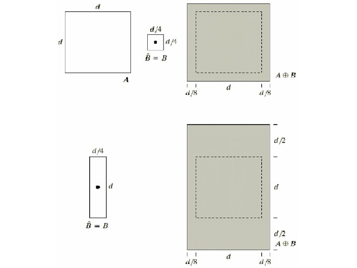
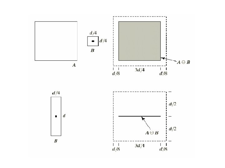
Erosion Definition Y=X _ B Example X Y mask B

More Erosion mask B X Y

Duality Between Erosion and Dilation (X _ B)c =Xc B^ Proof: (X _ B)c ={z | Bz A }c = {z | Bz Ac = }c = {z | Bz Ac } =Xc B^

Example Xc X B X _ B ^B Xc B^ (X _ B)c

Opening: Erosion + Dilation Definition (X _ B) B Example X _ mask B

Interpretation of Opening • Objects that are smaller than the SE will be removed, as well as “arms” from large objects that are narrower than the SE. • Noise Cleaning effect.

Closing: Dilation and Erosion Definition _ (X + B) B Example X + _ mask B

Interpretation of Closing • Holes in and around the object that are narrower than the SE will be filled up. • Noise Cleaning effect.

Properties of Opening and Closing Opening ● ● ● Closing ● ● ●

Effects of Opening and Closing

Simple Operations • Removing small objects by opening. • Filling small holes by closing. • Edge Detection: • Flood fill hollow A from point X 0 (Iteratively) • Continue until Xk=Xk-1. Filled A is • Connected component of point X 0

Binary Reconstruction Used after opening to grow back pieces of the original image that are connected to the opening. original opened reconstructed Removes of small regions that are disjoint from larger objects without distorting the small features of the large objects.

Medial Axis Morphology A B 4 B 8 Corners removed by first opening

Grayscale Morphology: Dilation Binary: Grey:

Grayscale Morphology: Erosion

Greyscale Morphology Applications • Noise Filtering (Salt & Pepper Noise) – Opening-Closing (min-max-min) • Edge Detection • Greyscale skeleton (Arithmetic operations!)