Binary Image Analysis Outline n n n Introduction

Binary Image Analysis

Outline n n n Introduction to binary image analysis Thresholding Mathematical morphology Pixels and neighborhoods Connected components analysis CS 484, Fall 2019 2

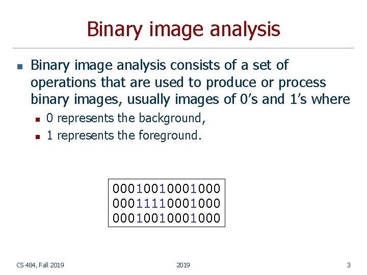
Binary image analysis n Binary image analysis consists of a set of operations that are used to produce or process binary images, usually images of 0’s and 1’s where n n 0 represents the background, 1 represents the foreground. 0001001000 0001111000 0001001000 CS 484, Fall 2019 3

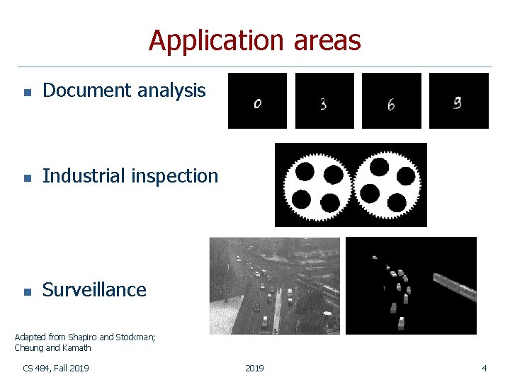
Application areas n Document analysis n Industrial inspection n Surveillance Adapted from Shapiro and Stockman; Cheung and Kamath CS 484, Fall 2019 4

Operations n Separate objects from background and from one another. n Aggregate pixels for each object. n Compute features for each object. CS 484, Fall 2019 5

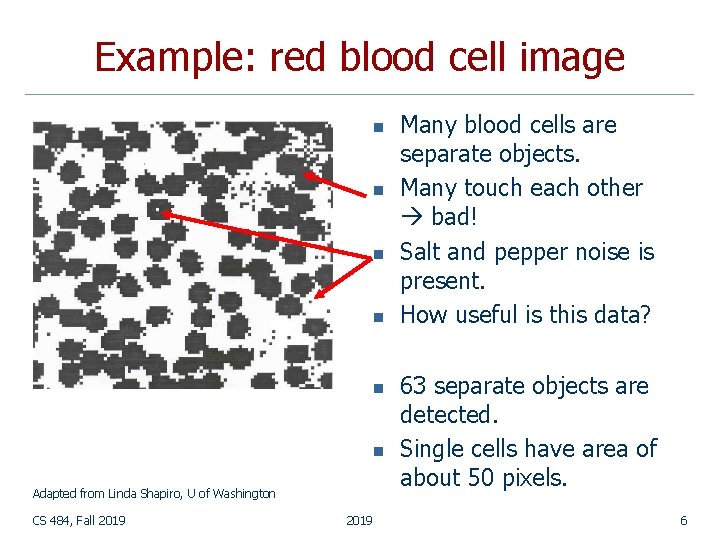
Example: red blood cell image n n n Adapted from Linda Shapiro, U of Washington CS 484, Fall 2019 Many blood cells are separate objects. Many touch each other bad! Salt and pepper noise is present. How useful is this data? 63 separate objects are detected. Single cells have area of about 50 pixels. 6

Thresholding n n Binary images can be obtained by thresholding. Assumptions for thresholding: n n Object region of interest has intensity distribution different from background. Object pixels likely to be identified by intensity alone: n n n intensity > a intensity < b a < intensity < b Works OK with flat-shaded scenes or engineered scenes. Does not work well with natural scenes. CS 484, Fall 2019 7

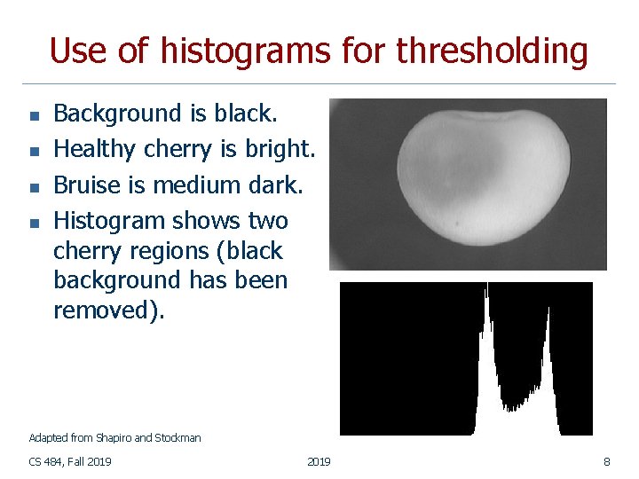
Use of histograms for thresholding n n Background is black. Healthy cherry is bright. Bruise is medium dark. Histogram shows two cherry regions (black background has been removed). Adapted from Shapiro and Stockman CS 484, Fall 2019 8

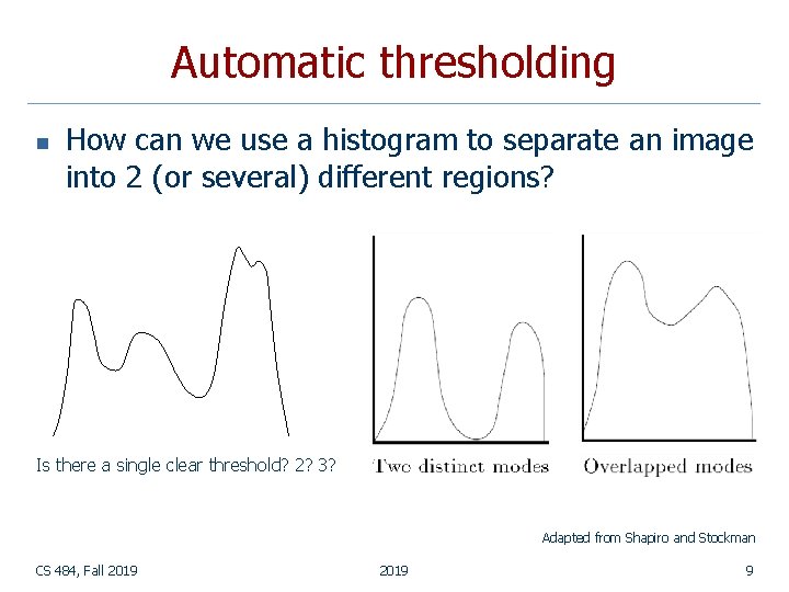
Automatic thresholding n How can we use a histogram to separate an image into 2 (or several) different regions? Is there a single clear threshold? 2? 3? Adapted from Shapiro and Stockman CS 484, Fall 2019 9

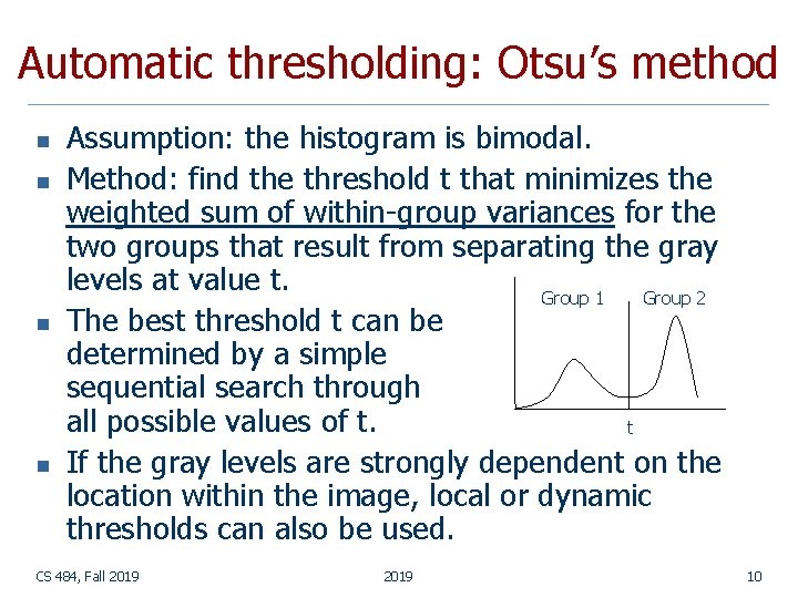
Automatic thresholding: Otsu’s method n n Assumption: the histogram is bimodal. Method: find the threshold t that minimizes the weighted sum of within-group variances for the two groups that result from separating the gray levels at value t. Group 1 Group 2 The best threshold t can be determined by a simple sequential search through all possible values of t. t If the gray levels are strongly dependent on the location within the image, local or dynamic thresholds can also be used. CS 484, Fall 2019 10

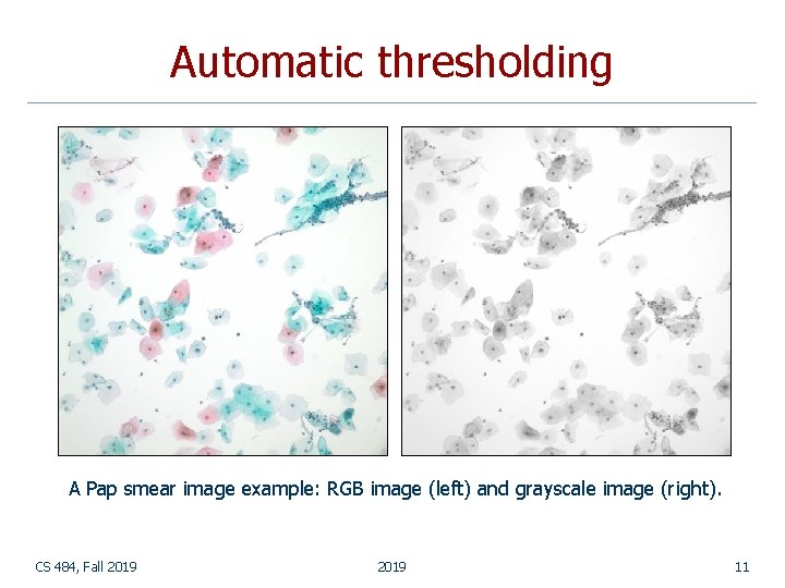
Automatic thresholding A Pap smear image example: RGB image (left) and grayscale image (right). CS 484, Fall 2019 11

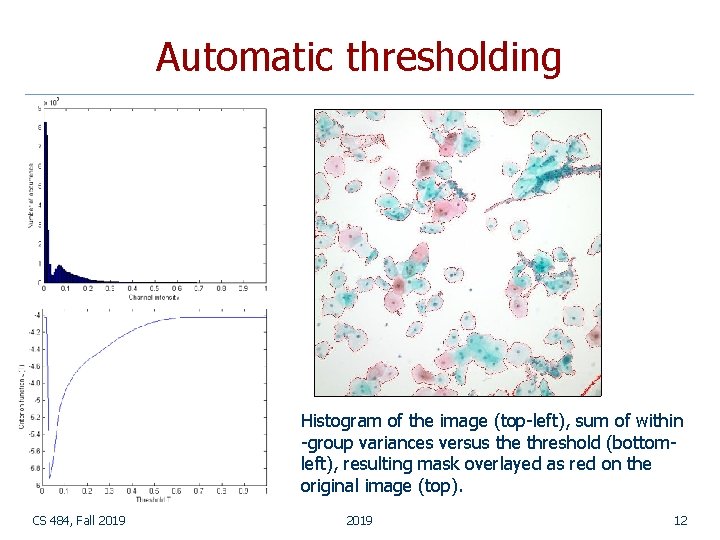
Automatic thresholding Histogram of the image (top-left), sum of within -group variances versus the threshold (bottomleft), resulting mask overlayed as red on the original image (top). CS 484, Fall 2019 12

Mathematical morphology n n The word morphology refers to form and structure. In computer vision, it is used to refer to the shape of a region. The language of mathematical morphology is set theory where sets represent objects in an image. We will discuss morphological operations on binary images whose components are sets in the 2 D integer space Z 2. CS 484, Fall 2019 13

Mathematical morphology n Mathematical morphology consists of two basic operations n n dilation erosion and several composite relations n n opening closing conditional dilation … CS 484, Fall 2019 14

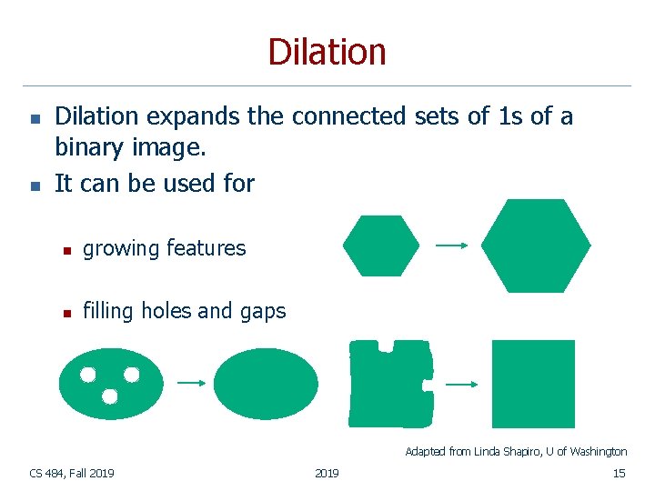
Dilation n n Dilation expands the connected sets of 1 s of a binary image. It can be used for n growing features n filling holes and gaps Adapted from Linda Shapiro, U of Washington CS 484, Fall 2019 15

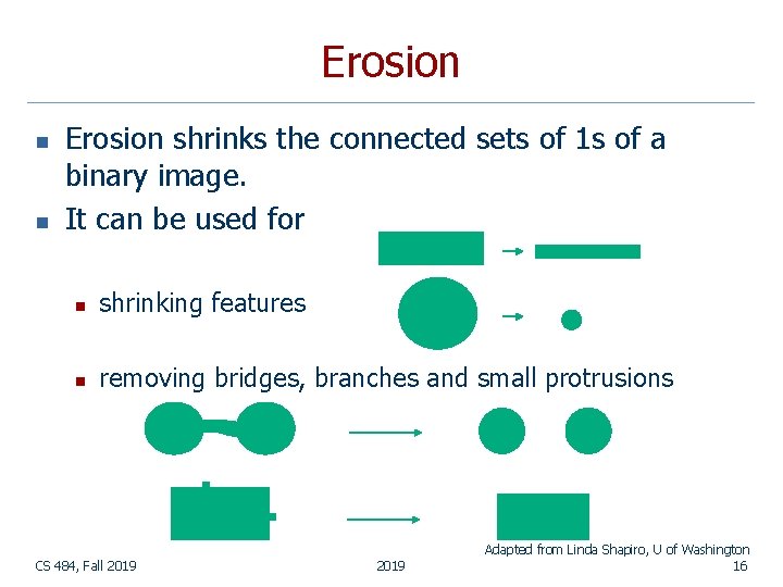
Erosion n n Erosion shrinks the connected sets of 1 s of a binary image. It can be used for n shrinking features n removing bridges, branches and small protrusions CS 484, Fall 2019 Adapted from Linda Shapiro, U of Washington 16

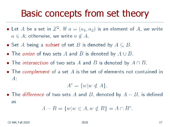
Basic concepts from set theory CS 484, Fall 2019 17

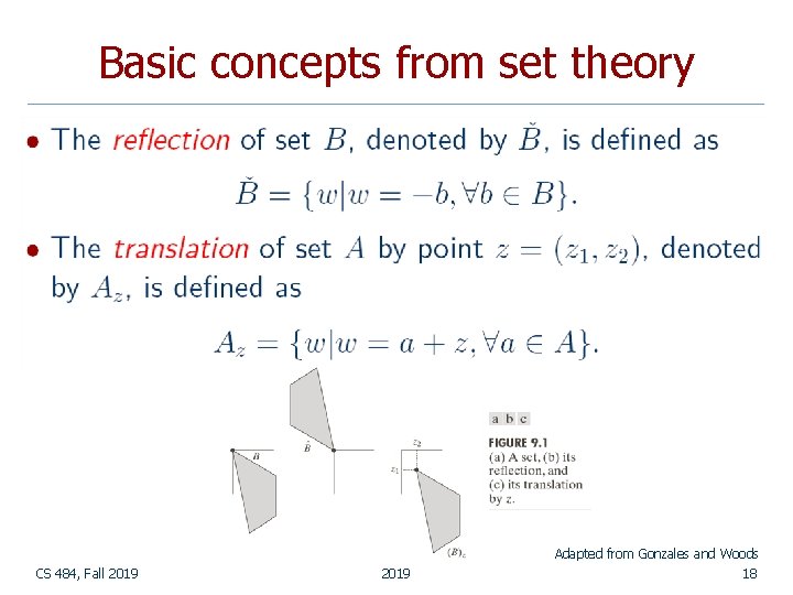
Basic concepts from set theory Adapted from Gonzales and Woods CS 484, Fall 2019 18

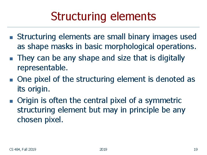
Structuring elements n n Structuring elements are small binary images used as shape masks in basic morphological operations. They can be any shape and size that is digitally representable. One pixel of the structuring element is denoted as its origin. Origin is often the central pixel of a symmetric structuring element but may in principle be any chosen pixel. CS 484, Fall 2019 19

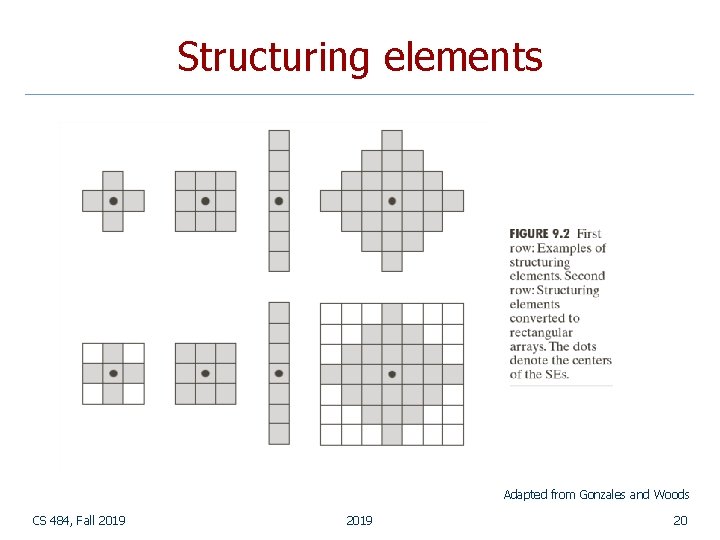
Structuring elements Adapted from Gonzales and Woods CS 484, Fall 2019 20

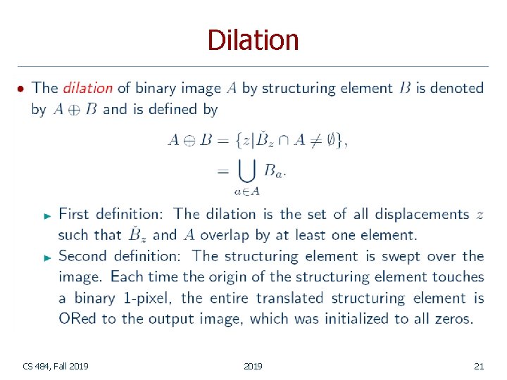
Dilation CS 484, Fall 2019 21

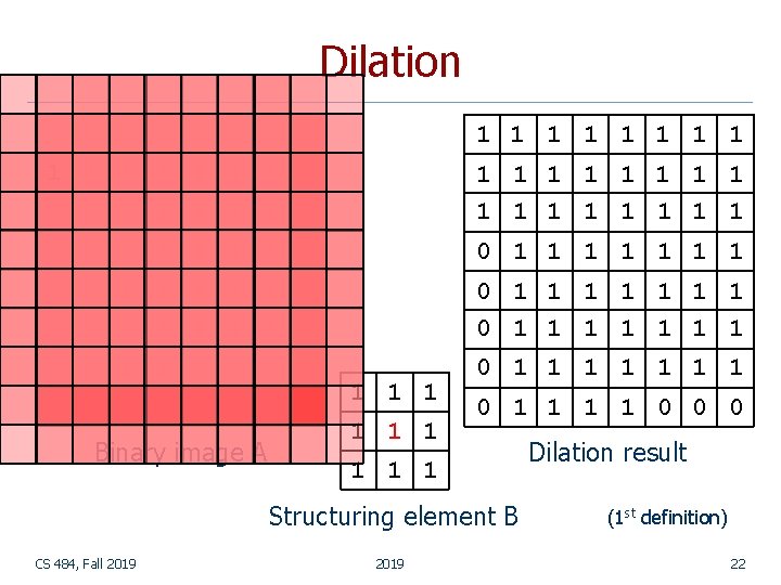
Dilation 1 1 1 1 1 1 1 1 1 1 1 1 1 0 1 1 1 1 Binary image A 0 1 1 1 1 0 1 1 1 1 0 0 0 Structuring element B CS 484, Fall 2019 Dilation result (1 st definition) 22

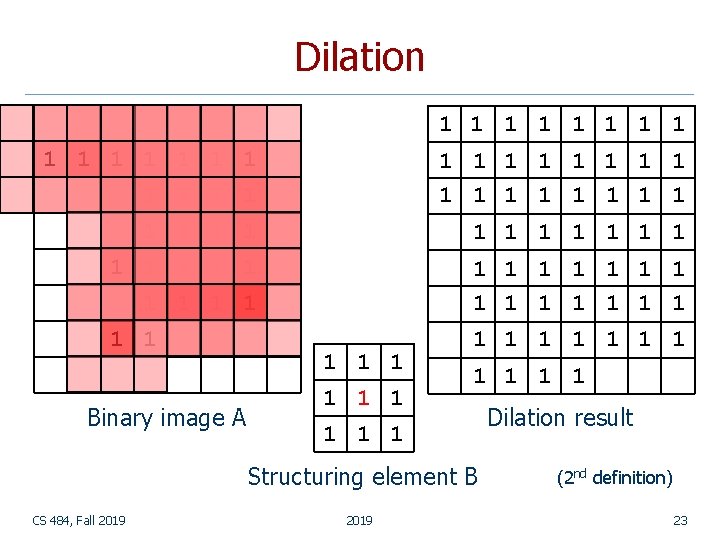
Dilation 1 1 1 1 1 1 1 1 1 1 1 1 1 1 1 1 Binary image A 1 1 1 1 1 1 1 Structuring element B CS 484, Fall 2019 Dilation result (2 nd definition) 23

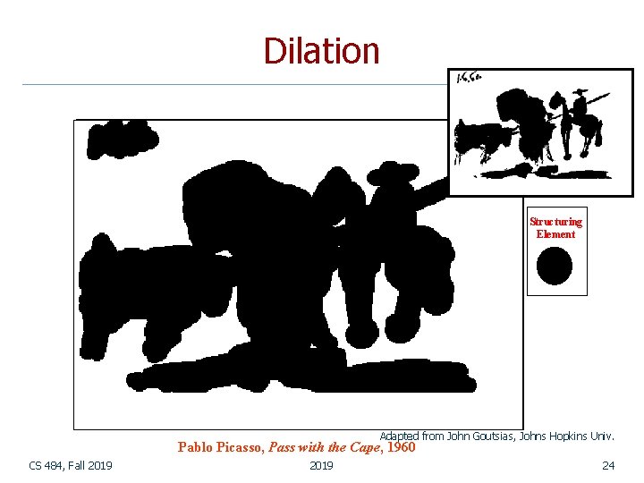
Dilation Structuring Element Adapted from John Goutsias, Johns Hopkins Univ. Pablo Picasso, Pass with the Cape, 1960 CS 484, Fall 2019 24

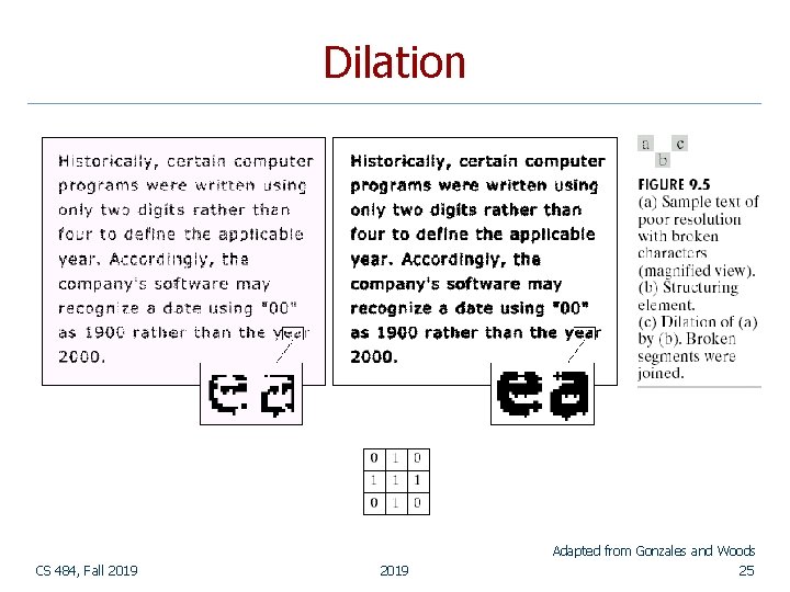
Dilation Adapted from Gonzales and Woods CS 484, Fall 2019 25

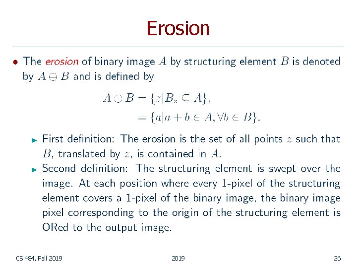
Erosion CS 484, Fall 2019 26

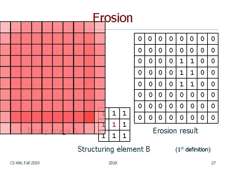
Erosion 0 0 0 0 1 1 1 1 0 0 0 1 1 0 0 1 1 1 0 0 1 1 0 0 0 0 0 Binary image A 0 0 1 1 1 1 1 0 0 0 0 Structuring element B CS 484, Fall 2019 Erosion result (1 st definition) 27

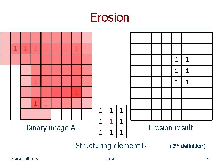
Erosion 1 1 1 1 1 1 1 Binary image A 1 1 1 1 Structuring element B CS 484, Fall 2019 Erosion result (2 nd definition) 28

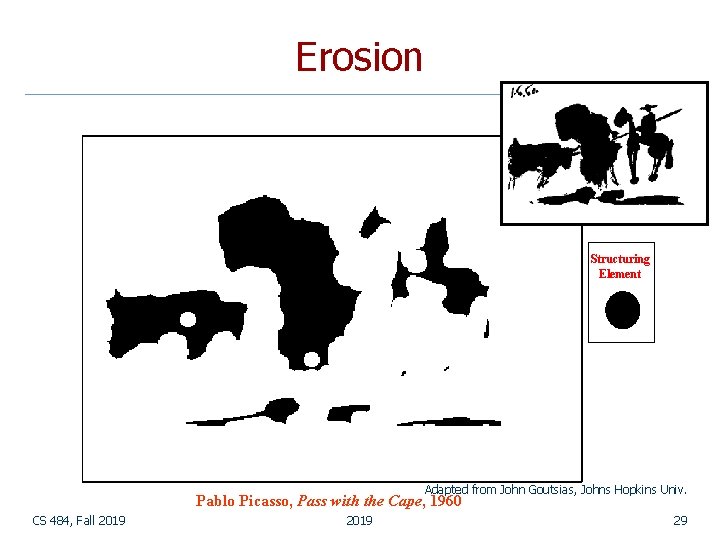
Erosion Structuring Element Adapted from John Goutsias, Johns Hopkins Univ. Pablo Picasso, Pass with the Cape, 1960 CS 484, Fall 2019 29

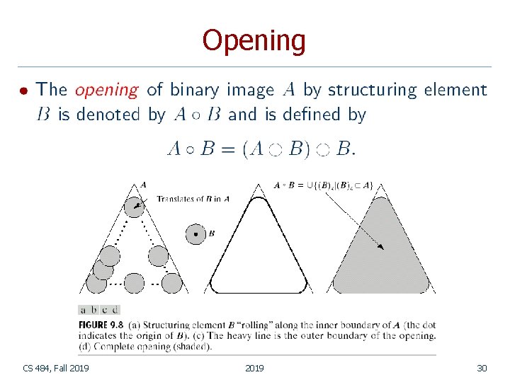
Opening CS 484, Fall 2019 30

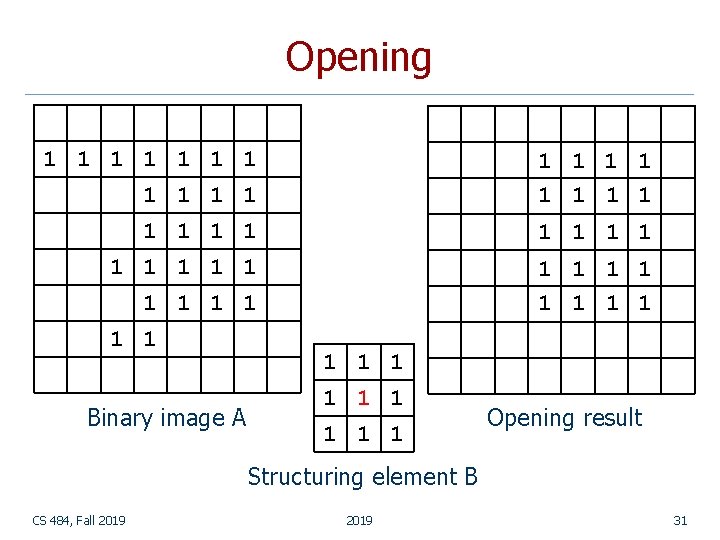
Opening 1 1 1 1 1 1 1 1 1 1 1 Binary image A 1 1 1 1 Opening result Structuring element B CS 484, Fall 2019 31

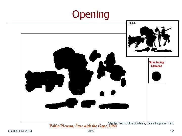
Opening Structuring Element Adapted from John Goutsias, Johns Hopkins Univ. Pablo Picasso, Pass with the Cape, 1960 CS 484, Fall 2019 32

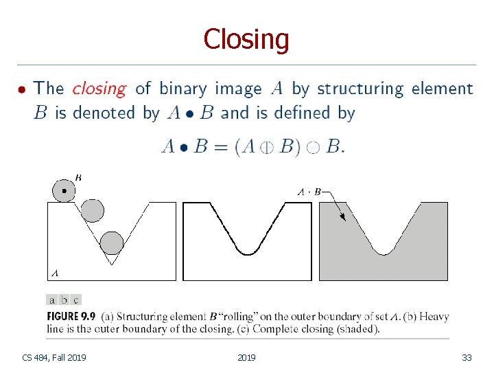
Closing CS 484, Fall 2019 33

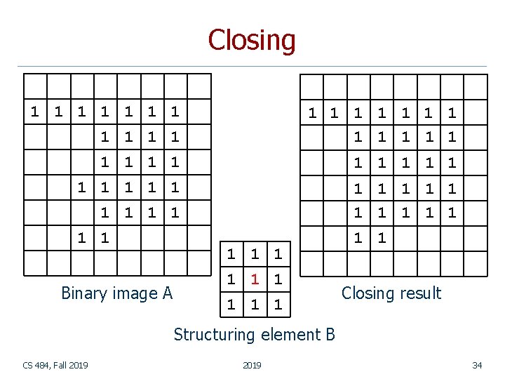
Closing 1 1 1 1 1 1 1 1 1 1 1 1 Binary image A 1 1 1 1 Closing result Structuring element B CS 484, Fall 2019 34

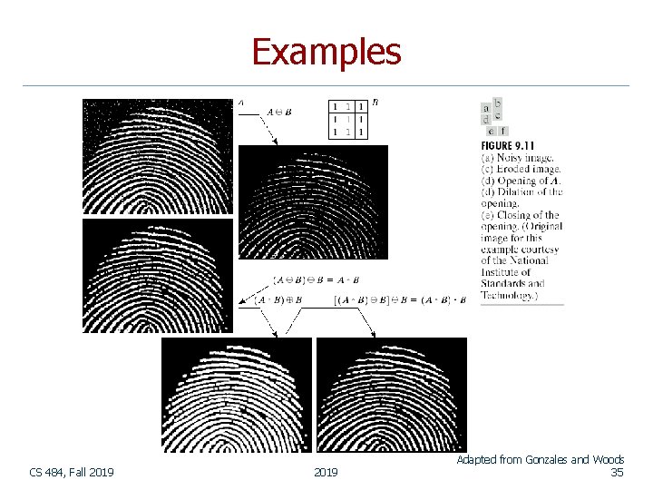
Examples CS 484, Fall 2019 Adapted from Gonzales and Woods 35

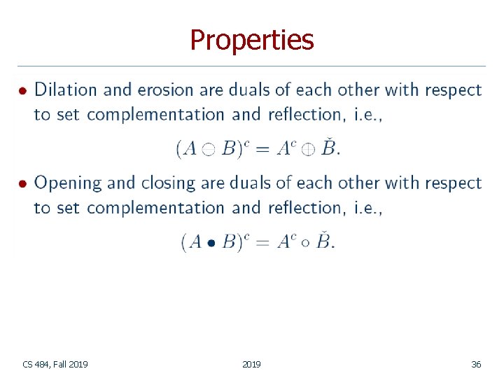
Properties CS 484, Fall 2019 36

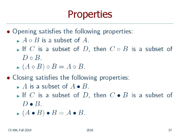
Properties CS 484, Fall 2019 37

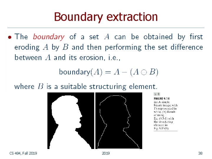
Boundary extraction CS 484, Fall 2019 38

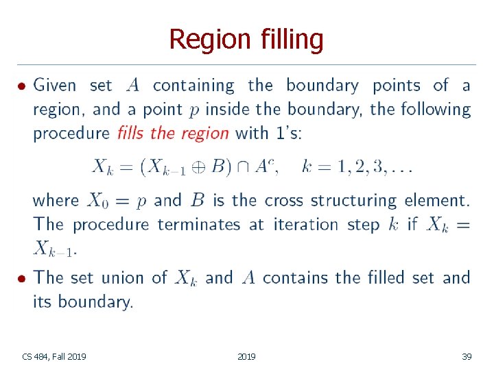
Region filling CS 484, Fall 2019 39

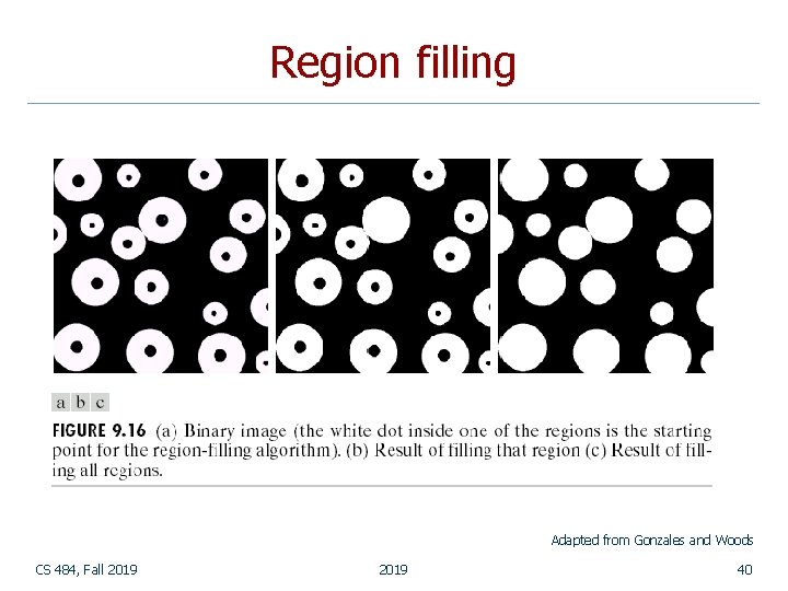
Region filling Adapted from Gonzales and Woods CS 484, Fall 2019 40

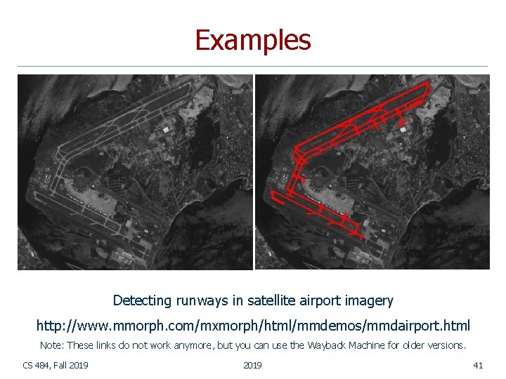
Examples Detecting runways in satellite airport imagery http: //www. mmorph. com/mxmorph/html/mmdemos/mmdairport. html Note: These links do not work anymore, but you can use the Wayback Machine for older versions. CS 484, Fall 2019 41

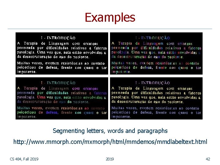
Examples Segmenting letters, words and paragraphs http: //www. mmorph. com/mxmorph/html/mmdemos/mmdlabeltext. html CS 484, Fall 2019 42

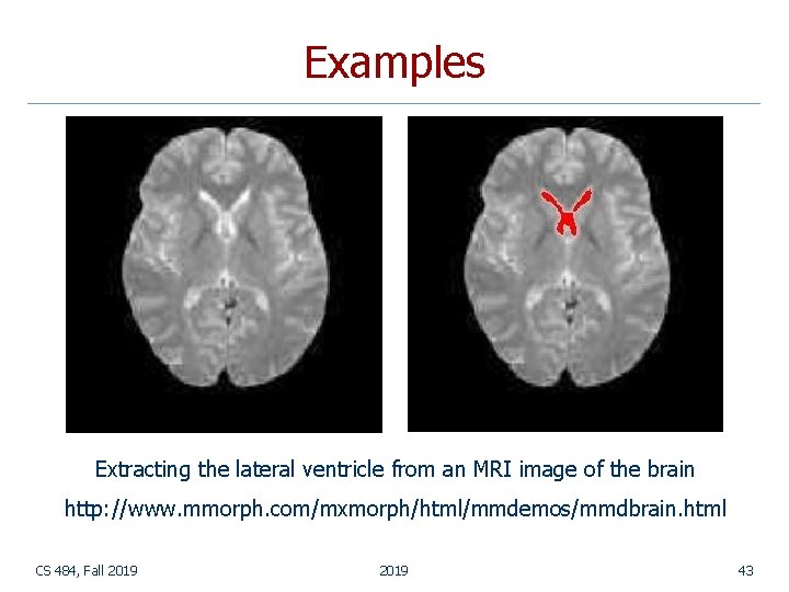
Examples Extracting the lateral ventricle from an MRI image of the brain http: //www. mmorph. com/mxmorph/html/mmdemos/mmdbrain. html CS 484, Fall 2019 43

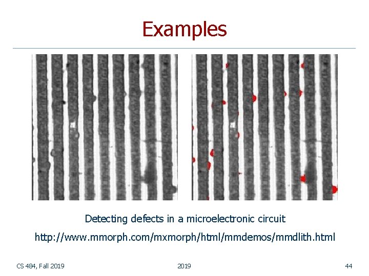
Examples Detecting defects in a microelectronic circuit http: //www. mmorph. com/mxmorph/html/mmdemos/mmdlith. html CS 484, Fall 2019 44

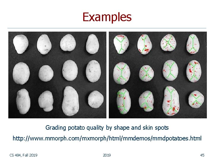
Examples Grading potato quality by shape and skin spots http: //www. mmorph. com/mxmorph/html/mmdemos/mmdpotatoes. html CS 484, Fall 2019 45

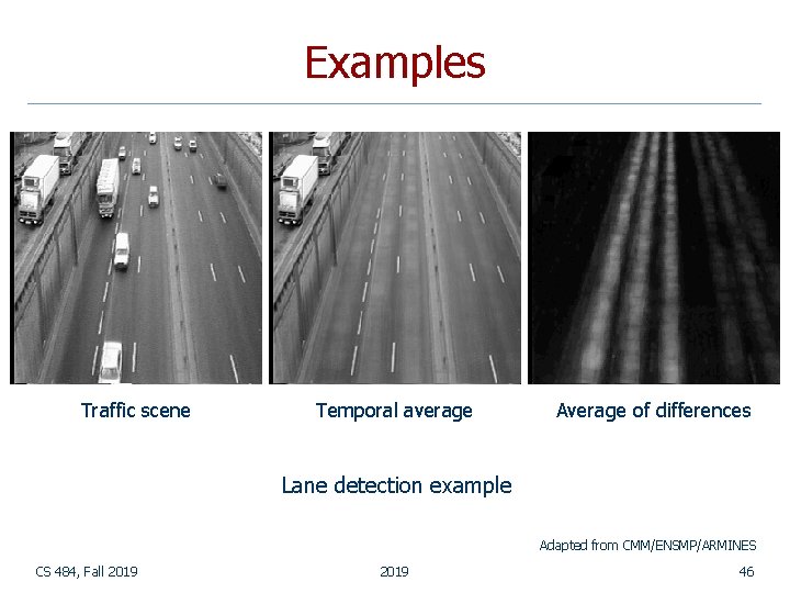
Examples Traffic scene Temporal average Average of differences Lane detection example Adapted from CMM/ENSMP/ARMINES CS 484, Fall 2019 46

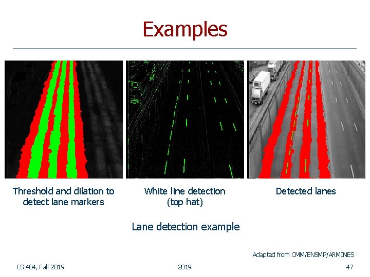
Examples Threshold and dilation to detect lane markers White line detection (top hat) Detected lanes Lane detection example Adapted from CMM/ENSMP/ARMINES CS 484, Fall 2019 47

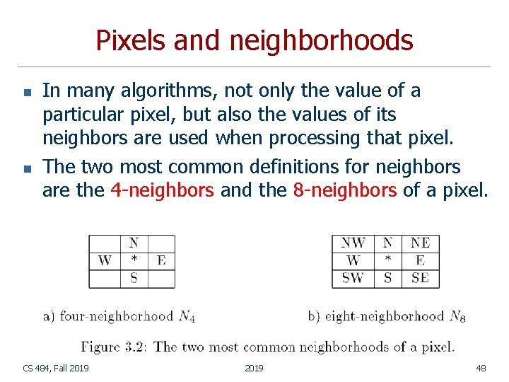
Pixels and neighborhoods n n In many algorithms, not only the value of a particular pixel, but also the values of its neighbors are used when processing that pixel. The two most common definitions for neighbors are the 4 -neighbors and the 8 -neighbors of a pixel. CS 484, Fall 2019 48

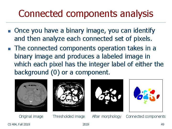
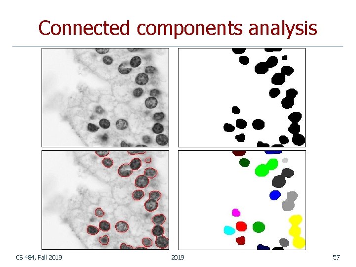
Connected components analysis n n Once you have a binary image, you can identify and then analyze each connected set of pixels. The connected components operation takes in a binary image and produces a labeled image in which each pixel has the integer label of either the background (0) or a component. Original image CS 484, Fall 2019 Thresholded image 2019 After morphology Connected components 49

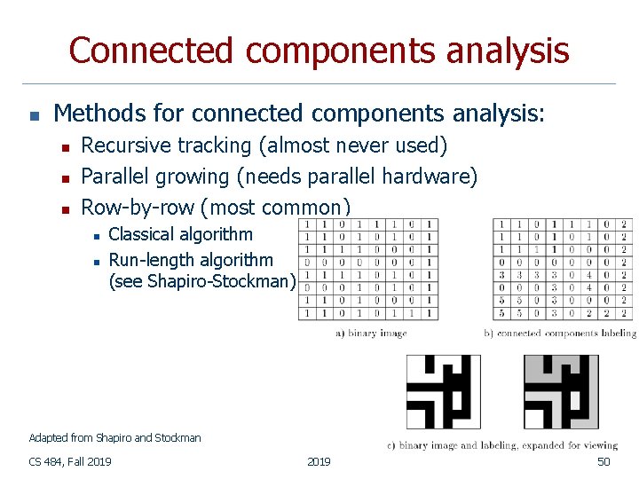
Connected components analysis n Methods for connected components analysis: n n n Recursive tracking (almost never used) Parallel growing (needs parallel hardware) Row-by-row (most common) n n Classical algorithm Run-length algorithm (see Shapiro-Stockman) Adapted from Shapiro and Stockman CS 484, Fall 2019 50

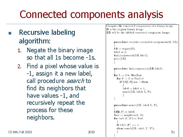
Connected components analysis n Recursive labeling algorithm: Negate the binary image so that all 1 s become -1 s. 2. Find a pixel whose value is -1, assign it a new label, call procedure search to find its neighbors that have values -1, and recursively repeat the process for these neighbors. 1. CS 484, Fall 2019 51

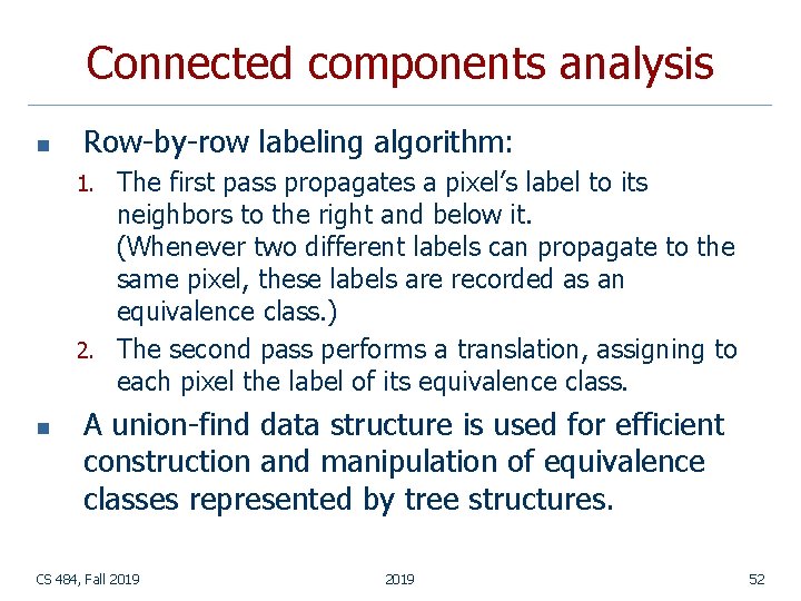
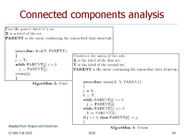
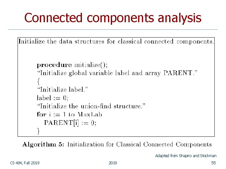
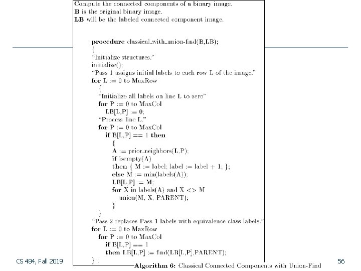
Connected components analysis n Row-by-row labeling algorithm: The first pass propagates a pixel’s label to its neighbors to the right and below it. (Whenever two different labels can propagate to the same pixel, these labels are recorded as an equivalence class. ) 2. The second pass performs a translation, assigning to each pixel the label of its equivalence class. 1. n A union-find data structure is used for efficient construction and manipulation of equivalence classes represented by tree structures. CS 484, Fall 2019 52

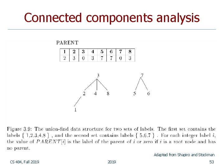
Connected components analysis Adapted from Shapiro and Stockman CS 484, Fall 2019 53

Connected components analysis Adapted from Shapiro and Stockman CS 484, Fall 2019 54

Connected components analysis Adapted from Shapiro and Stockman CS 484, Fall 2019 55

CS 484, Fall 2019 56

Connected components analysis CS 484, Fall 2019 57

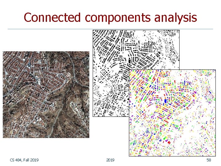
Connected components analysis CS 484, Fall 2019 58