Binary Decision Diagrams Giovanni De Micheli Integrated Systems

Binary Decision Diagrams Giovanni De Micheli Integrated Systems Laboratory This presentation can be used for non-commercial purposes as long as this note and the copyright footers are not removed © Giovanni De Micheli – All rights reserved
Module 1 u Objectives: s Definitions of BDDs, OBDDs and ROBDDs s Logic operations on BDDs s The ITE operator (c) Giovanni De Micheli 2
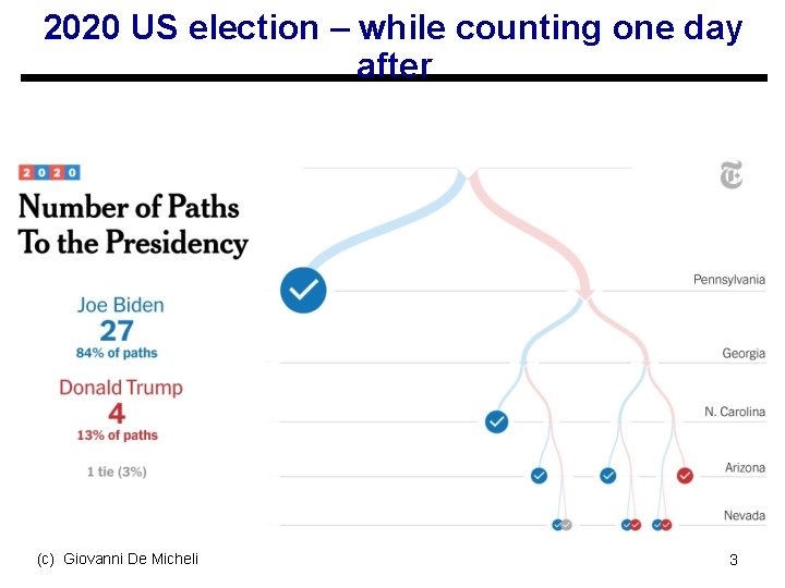
2020 US election – while counting one day after (c) Giovanni De Micheli 3
Motivation u Efficient way to represent logic functions u History s Original idea for BDD due to Lee (1959) and Akers (1978) s Refined, formalized and popularized by Bryant (1986) t t Smaller memory footprint Canonical form – each distinct function correspond to a unique distinct diagram (c) Giovanni De Micheli 6
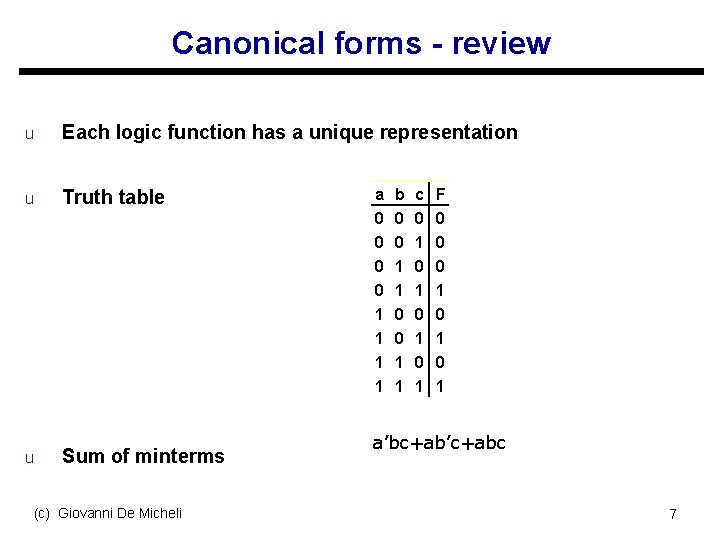
Canonical forms - review u Each logic function has a unique representation u Truth table u Sum of minterms (c) Giovanni De Micheli a 0 0 1 1 b 0 0 1 1 c 0 1 0 1 F 0 0 0 1 0 1 a’bc+ab’c+abc 7
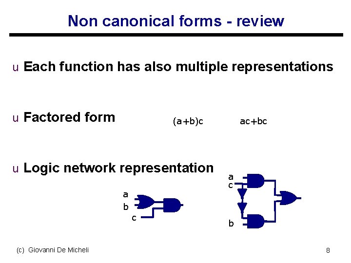
Non canonical forms - review u Each function has also multiple representations u Factored form (a+b)c u Logic network representation a b c (c) Giovanni De Micheli ac+bc a c b 8
Terminology u A Binary Decision Diagram (BDD) is a directed acyclic graph s Graph: set of vertices connected by edges s Directed: edges have direction s Acyclic: no path in the graph can lead to a cycle u Often abbreviated as DAG s Simplest model: t t t Two leaves (Boolean constants 0 and 1) One root Can degenerate to a tree (c) Giovanni De Micheli 9
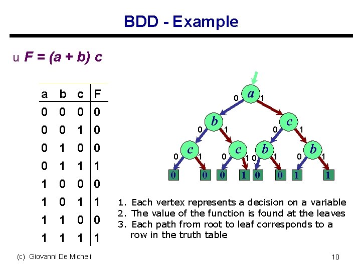
BDD - Example u F = (a + b) c a 0 0 1 1 b 0 0 1 1 c 0 1 0 1 (c) Giovanni De Micheli F 0 0 0 1 0 1 a 0 0 c 1 0 b 1 1 0 0 0 c 10 1 0 b 1 0 c 1 0 1 b 1 1 1. Each vertex represents a decision on a variable 2. The value of the function is found at the leaves 3. Each path from root to leaf corresponds to a row in the truth table 10
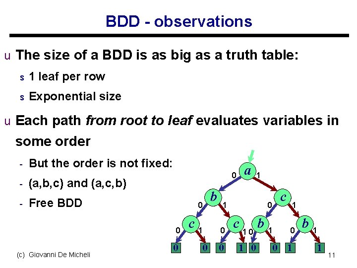
BDD - observations u The size of a BDD is as big as a truth table: s 1 leaf per row s Exponential size u Each path from root to leaf evaluates variables in some order - But the order is not fixed: - (a, b, c) and (a, c, b) - Free BDD 0 0 (c) Giovanni De Micheli a 0 0 c 1 0 b 1 0 0 1 0 c 10 1 0 b 1 c 1 0 0 1 b 1 1 11
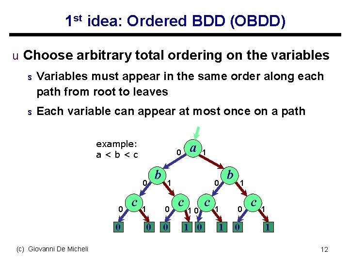
1 st idea: Ordered BDD (OBDD) u Choose arbitrary total ordering on the variables s Variables must appear in the same order along each path from root to leaves s Each variable can appear at most once on a path example: a<b<c 0 0 0 (c) Giovanni De Micheli c a 0 1 0 b 1 1 0 0 0 c 10 1 0 c 1 1 b 1 0 0 c 1 1 12
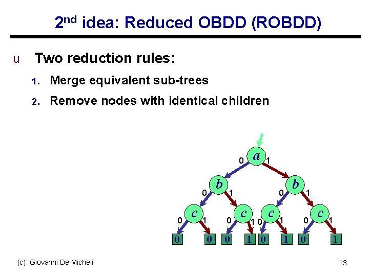
2 nd idea: Reduced OBDD (ROBDD) u Two reduction rules: 1. Merge equivalent sub-trees 2. Remove nodes with identical children a 0 0 (c) Giovanni De Micheli c 1 0 b 1 1 0 0 0 c 10 1 0 c 1 1 b 1 0 0 c 1 1 13
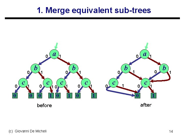
1. Merge equivalent sub-trees a 0 0 c 1 0 b 1 1 0 0 0 c 0 10 1 0 before (c) Giovanni De Micheli c 1 1 b 1 0 0 0 c 1 1 0 c b 1 a 1 1 0 0 c b 1 1 0 1 after 14
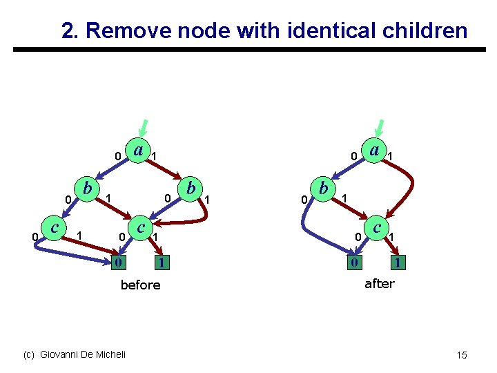
2. Remove node with identical children 0 0 0 c b 1 a 1 0 0 0 c 1 1 before (c) Giovanni De Micheli b 1 0 b a 1 1 0 0 c 1 1 after 15
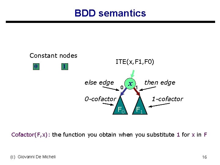
BDD semantics Constant nodes 0 ITE(x, F 1, F 0) 1 else edge 0 x 1 0 -cofactor then edge 1 -cofactor F 0 F 1 Cofactor(F, x): the function you obtain when you substitute 1 for x in F (c) Giovanni De Micheli 16
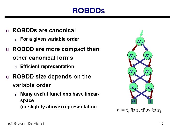
ROBDDs u ROBDDs are canonical s For a given variable order u ROBDD are more compact than other canonical forms s Efficient representation u ROBDD size depends on the variable order s Many useful functions have linearspace (or slightly above) representation (c) Giovanni De Micheli x 1 x 2 x 3 x 4 0 1 17
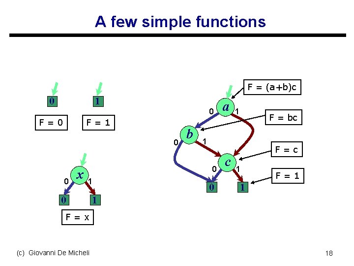
A few simple functions F = (a+b)c 0 1 F=0 F=1 0 0 0 x b 0 1 F = bc 1 0 1 a 0 c F=c 1 F=1 1 1 F=x (c) Giovanni De Micheli 18
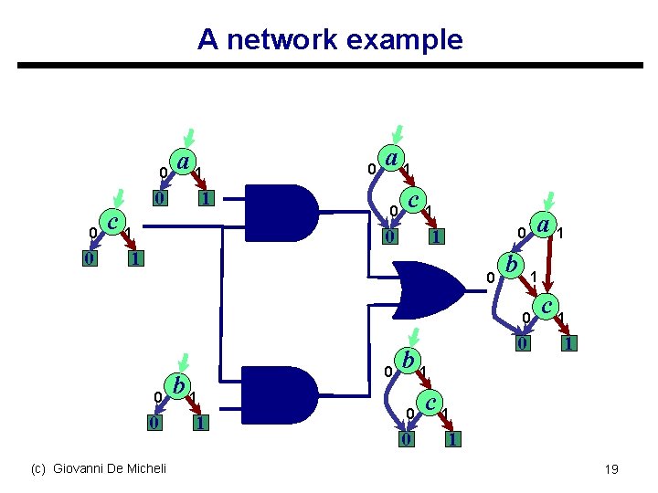
A network example 0 0 0 c 1 a 1 0 c 1 0 a 1 0 1 1 0 b 1 0 0 0 (c) Giovanni De Micheli b 1 1 0 0 b 1 0 0 c 1 1 19
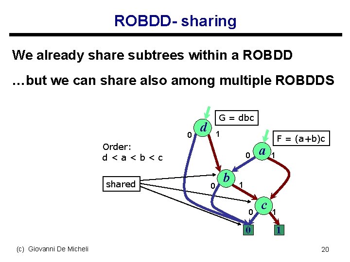
ROBDD- sharing We already share subtrees within a ROBDD …but we can share also among multiple ROBDDS 0 G = dbc d 1 Order: d<a<b<c shared 0 0 b 1 1 0 0 (c) Giovanni De Micheli a F = (a+b)c c 1 1 20
ROBDDs- why do we care ? u Easy to solve some important problems: 1. Tautology checking Just check if BDD is identical to function 2. Identity checking: F = G 3. Satisfiability 1 Look for a path from root to leaf 1 u All while having a compact representation s Use small memory footprint (c) Giovanni De Micheli 21
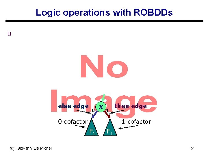
Logic operations with ROBDDs u else edge 0 x 1 0 -cofactor 1 -cofactor F 0 (c) Giovanni De Micheli then edge F 1 22
Logic operations with ROBDDs u (c) Giovanni De Micheli 23
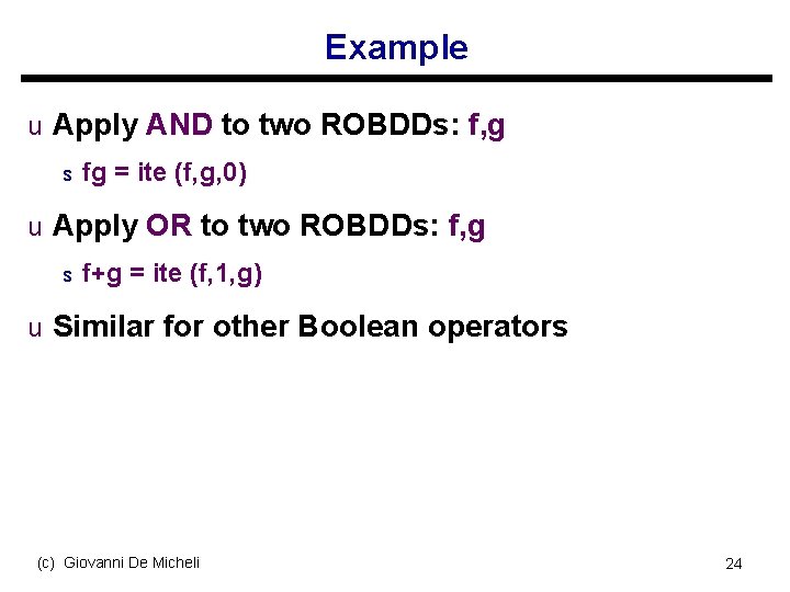
Example u Apply AND to two ROBDDs: f, g s fg = ite (f, g, 0) u Apply OR to two ROBDDs: f, g s f+g = ite (f, 1, g) u Similar for other Boolean operators (c) Giovanni De Micheli 24
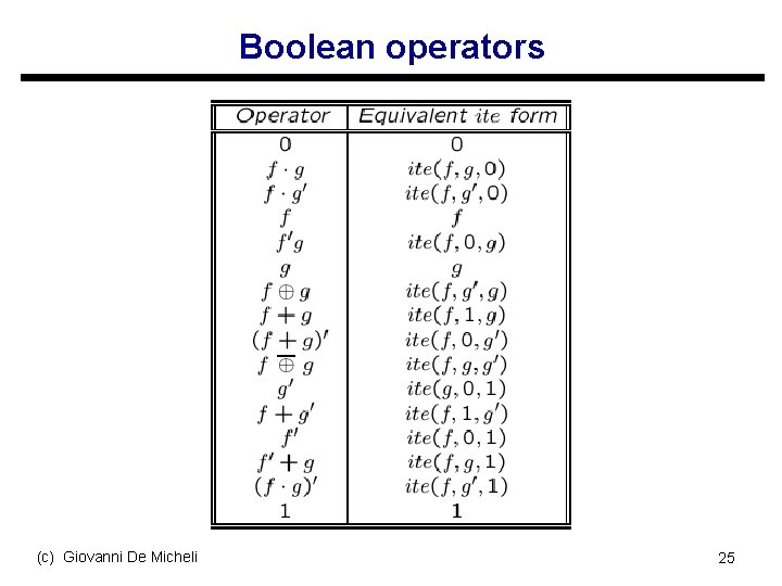
Boolean operators (c) Giovanni De Micheli 25
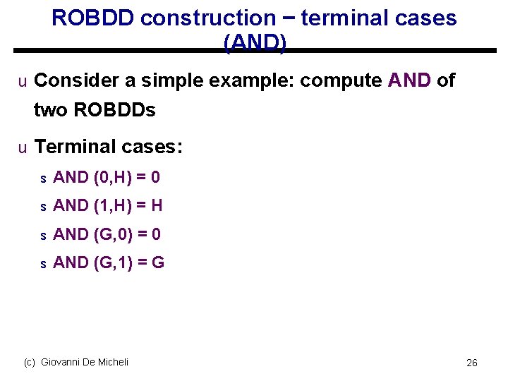
ROBDD construction – terminal cases (AND) u Consider a simple example: compute AND of two ROBDDs u Terminal cases: s AND (0, H) = 0 s AND (1, H) = H s AND (G, 0) = 0 s AND (G, 1) = G (c) Giovanni De Micheli 26
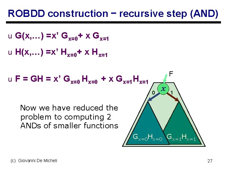
ROBDD construction – recursive step (AND) u G(x, …) =x’ Gx=0+ x Gx=1 u H(x, …) =x’ Hx=0+ x Hx=1 F u F = GH = x’ Gx=0 Hx=0 + x Gx=1 Hx=1 0 x 1 Now we have reduced the problem to computing 2 ANDs of smaller functions Gx=0 Hx=0 Gx=1 Hx=1 (c) Giovanni De Micheli 27
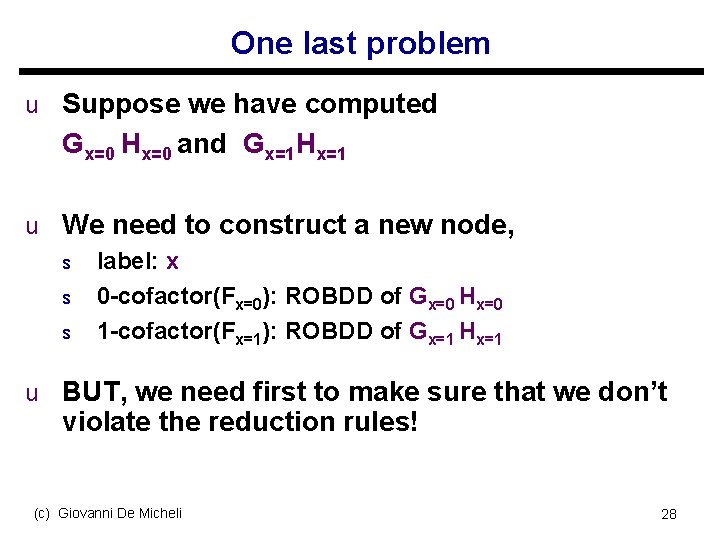
One last problem u Suppose we have computed Gx=0 Hx=0 and Gx=1 Hx=1 u We need to construct a new node, s label: x s 0 -cofactor(Fx=0): ROBDD of Gx=0 Hx=0 s 1 -cofactor(Fx=1): ROBDD of Gx=1 Hx=1 u BUT, we need first to make sure that we don’t violate the reduction rules! (c) Giovanni De Micheli 28
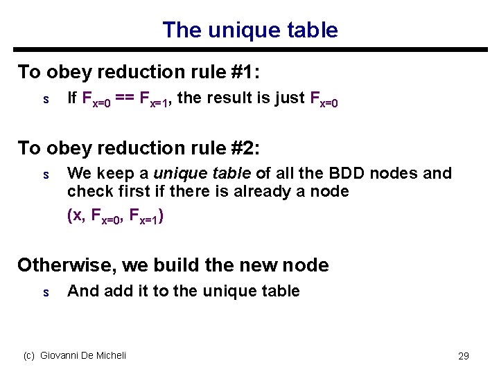
The unique table To obey reduction rule #1: s If Fx=0 == Fx=1, the result is just Fx=0 To obey reduction rule #2: s We keep a unique table of all the BDD nodes and check first if there is already a node (x, Fx=0, Fx=1) Otherwise, we build the new node s And add it to the unique table (c) Giovanni De Micheli 29
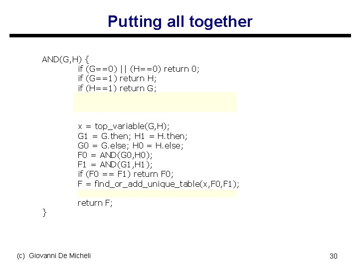
Putting all together AND(G, H) { if (G==0) || (H==0) return 0; if (G==1) return H; if (H==1) return G; cmp = computed_table_lookup(G, H); if (cmp != NULL) return cmp; } x = top_variable(G, H); G 1 = G. then; H 1 = H. then; G 0 = G. else; H 0 = H. else; F 0 = AND(G 0, H 0); F 1 = AND(G 1, H 1); if (F 0 == F 1) return F 0; F = find_or_add_unique_table(x, F 0, F 1); computed_table_insert(G, H, F); return F; (c) Giovanni De Micheli 30
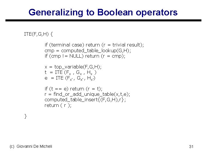
Generalizing to Boolean operators ITE(F, G, H) { if (terminal case) return (r = trivial result); cmp = computed_table_lookup(G, H); if (cmp != NULL) return (r = cmp); x = top_variable(F, G, H); t = ITE (Fx , Gx , Hx ) e = ITE (Fx’ , Gx’ , Hx’) if (t == e) return (r = t); r = find_or_add_unique_table(x, t, e); computed_table_insert{(F, G, H), r}; return ( r ); } (c) Giovanni De Micheli 31
Logic operations - summary u Recursive routines – traverse the DAGs depth first u Two tables: s Unique table – hash table with an entry for each BDD node s Computed table – store previously-computed partial results u Time complexity is quadratic in the BDD sizes (c) Giovanni De Micheli 32
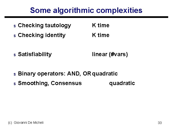
Some algorithmic complexities s Checking tautology K time s Checking identity K time s Satisfiability linear (#vars) s Binary operators: AND, OR quadratic s Smoothing, Consensus (c) Giovanni De Micheli quadratic 33
Motivation - again u Why are ROBDD popular? s Several intractable problems can be solved in polynomial time t s Of the BDD size In several cases, the BDD sizes grow mildly with the problem size t Variables u This does not mean that BDD solve intractable problems in polynomial time s Few counterexamples exists (c) Giovanni De Micheli 34
Module 2 u Objectives: s Variable ordering (static and dynamic) s Other diagrams and applications (c) Giovanni De Micheli 35
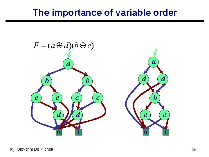
The importance of variable order a a b c (c) Giovanni De Micheli d b c d c c d d c c 0 1 b 36
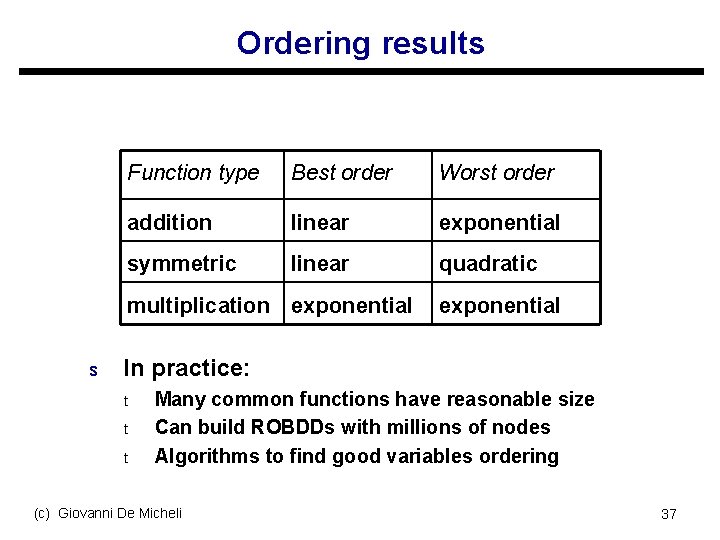
Ordering results Function type Best order Worst order addition linear exponential symmetric linear quadratic multiplication exponential s exponential In practice: t t t Many common functions have reasonable size Can build ROBDDs with millions of nodes Algorithms to find good variables ordering (c) Giovanni De Micheli 37
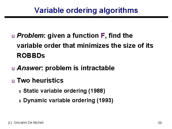
Variable ordering algorithms u Problem: given a function F, find the variable order that minimizes the size of its ROBBDs u Answer: problem is intractable u Two heuristics s Static variable ordering (1988) s Dynamic variable ordering (1993) (c) Giovanni De Micheli 38
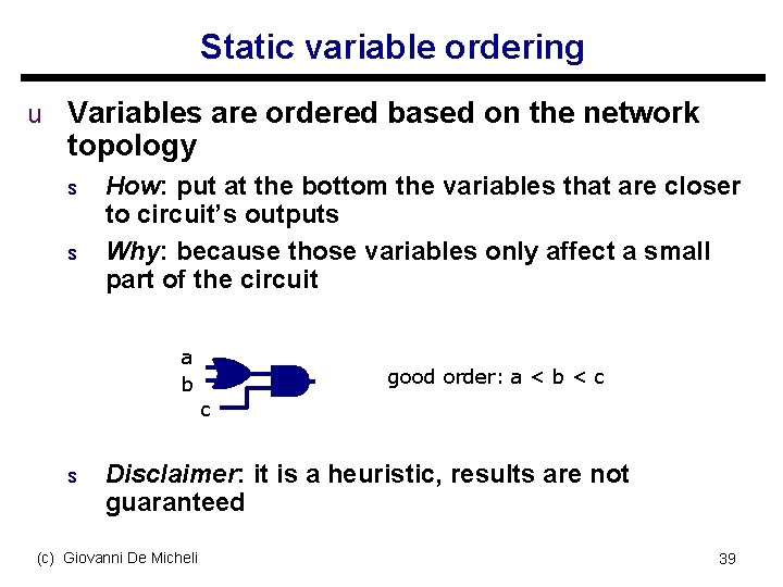
Static variable ordering u Variables are ordered based on the network topology s s How: put at the bottom the variables that are closer to circuit’s outputs Why: because those variables only affect a small part of the circuit a b good order: a < b < c c s Disclaimer: it is a heuristic, results are not guaranteed (c) Giovanni De Micheli 39
Dynamic variable ordering u Changes the variable order on the fly whenever ROBDDs become too big u How: trial and error – sifting algorithm Choose a variable 2. Move it in all possible positions of the variable order 3. Pick the position that leaves you with the smallest ROBDDs 4. Choose another variable … 1. (c) Giovanni De Micheli 40
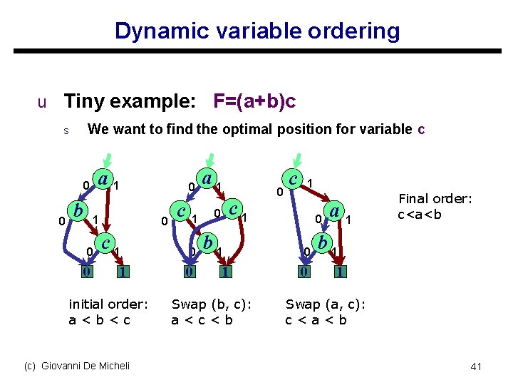
Dynamic variable ordering u Tiny example: F=(a+b)c We want to find the optimal position for variable c s a 1 0 0 b 1 0 0 0 c 1 1 initial order: a<b<c (c) Giovanni De Micheli c 0 a 1 1 0 0 b 1 0 c 1 1 Swap (b, c): a<c<b 0 c 1 0 0 0 a 1 Final order: c<a<b b 1 1 Swap (a, c): c<a<b 41
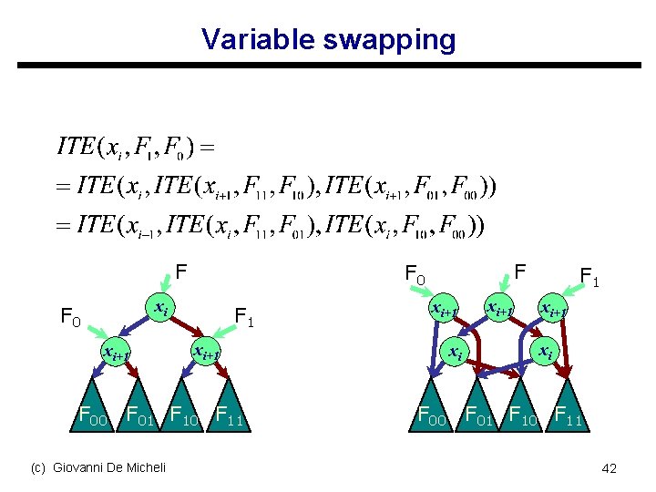
Variable swapping F xi F 0 xi+1 F 1 xi+1 F 00 F 01 F 10 F 11 (c) Giovanni De Micheli F F 0 xi+1 xi xi+1 F 1 xi+1 xi F 00 F 01 F 10 F 11 42
Dynamic variable ordering u Key idea: swapping two variables can be done locally s Efficient: t s Robust: t s It can be done just by sweeping the unique table It works well on many more circuits Warning: t t It is still non optimal At convergence, you most probably have found only a local minimum (c) Giovanni De Micheli 43
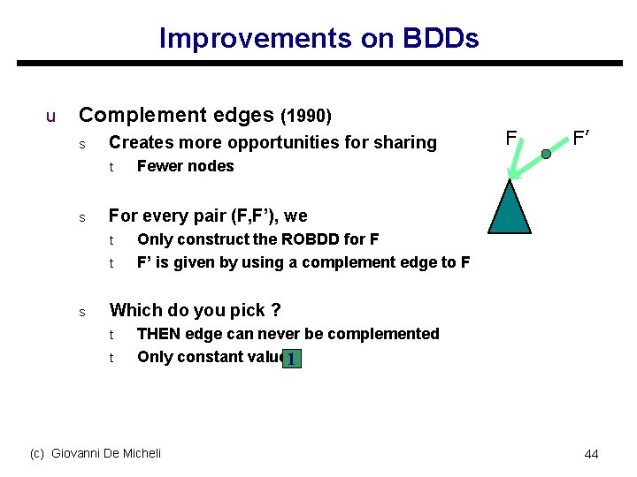
Improvements on BDDs u Complement edges (1990) s Creates more opportunities for sharing t s F’ Fewer nodes For every pair (F, F’), we t t s F Only construct the ROBDD for F F’ is given by using a complement edge to F Which do you pick ? t t THEN edge can never be complemented Only constant value 1 (c) Giovanni De Micheli 44
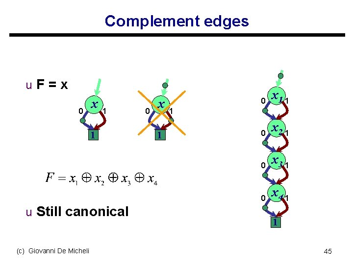
Complement edges u F = x 0 x 1 1 u Still canonical (c) Giovanni De Micheli 0 x 1 1 0 x 2 1 0 x 3 1 0 x 4 1 1 1 45
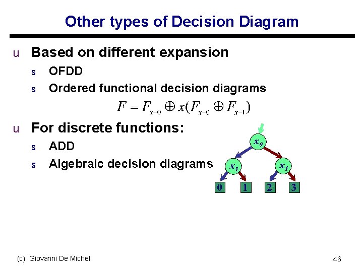
Other types of Decision Diagram u Based on different expansion s OFDD s Ordered functional decision diagrams u For discrete functions: s ADD s Algebraic decision diagrams x 0 0 (c) Giovanni De Micheli x 1 1 2 3 46
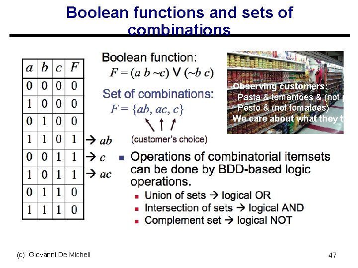
Boolean functions and sets of combinations Observing customers: Pasta & tomantoes & (not pest Pesto & (not tomatoes) We care about what they take (c) Giovanni De Micheli 47
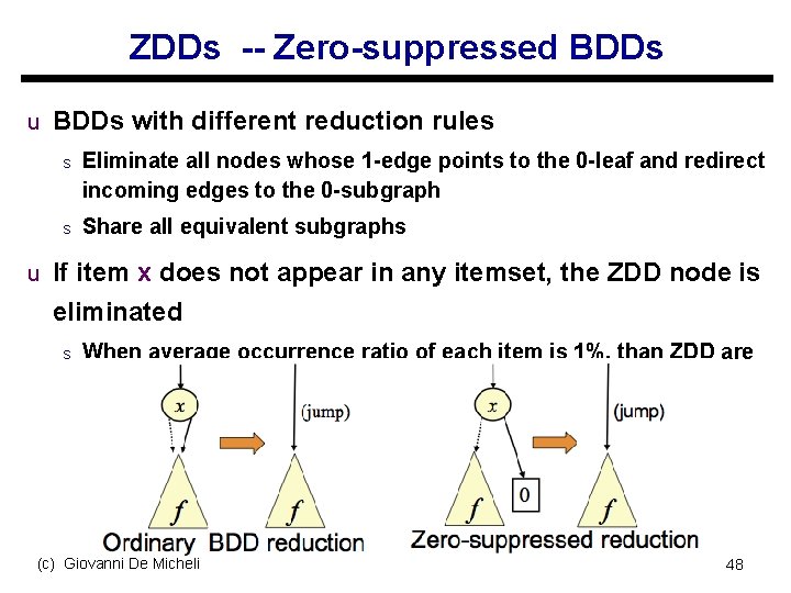
ZDDs -- Zero-suppressed BDDs u BDDs with different reduction rules s Eliminate all nodes whose 1 -edge points to the 0 -leaf and redirect incoming edges to the 0 -subgraph s Share all equivalent subgraphs u If item x does not appear in any itemset, the ZDD node is eliminated s When average occurrence ratio of each item is 1%, than ZDD are more efficient than BDDs (up to 100 times) (c) Giovanni De Micheli 48
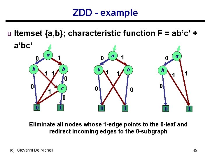
ZDD - example u Itemset {a, b}; characteristic function F = ab’c’ + a’bc’ 0 b a 1 0 b 1 0 c a 1 b 1 0 a 0 b 0 1 1 0 0 1 0 1 Eliminate all nodes whose 1 -edge points to the 0 -leaf and redirect incoming edges to the 0 -subgraph (c) Giovanni De Micheli 49
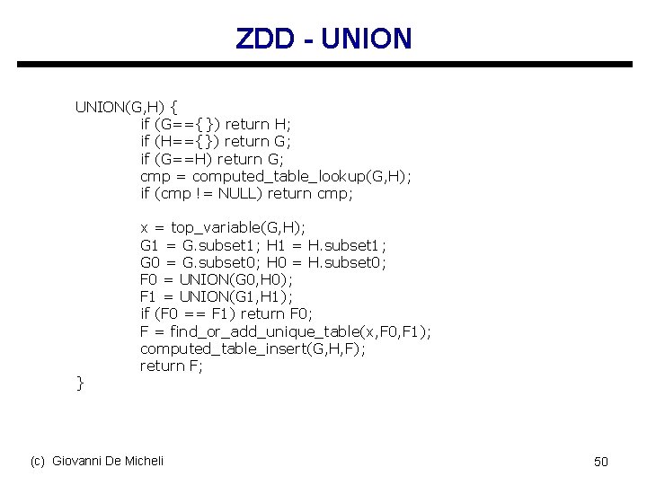
ZDD - UNION(G, H) { if (G=={}) return H; if (H=={}) return G; if (G==H) return G; cmp = computed_table_lookup(G, H); if (cmp != NULL) return cmp; } x = top_variable(G, H); G 1 = G. subset 1; H 1 = H. subset 1; G 0 = G. subset 0; H 0 = H. subset 0; F 0 = UNION(G 0, H 0); F 1 = UNION(G 1, H 1); if (F 0 == F 1) return F 0; F = find_or_add_unique_table(x, F 0, F 1); computed_table_insert(G, H, F); return F; (c) Giovanni De Micheli 50
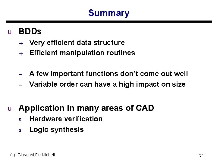
Summary u BDDs + Very efficient data structure + Efficient manipulation routines – – A few important functions don’t come out well Variable order can have a high impact on size u Application in many areas of CAD s Hardware verification s Logic synthesis (c) Giovanni De Micheli 51
- Slides: 49