Bin Packing Problem A parallel implementation By Christos

Bin Packing Problem: A parallel implementation By Christos Giavroudis Dissertation submitted in partial fulfilment for the degree of Master of Science in Communication & Information Systems Department of Informatics & Communications TEI of Central Macedonia

Bin Packing Problem: Definition � Suppose you need to place small objects in large containers with fixed size in order to have the minimum possible space, to use the fewest containers and the whole process can be done as soon as possible. � It is an optimization problem and belongs to combinatorial NP-hard problem

Bin Packing Problem: Definition � There is a list of numbers called “weights” � These numbers represent objects that need to be packed into “bins” with a particular capacity � The goal is to pack the weights into the smallest number of bins possible

Bin Packing Problem: Applications They have many applications, such as: � � � Objects coming down a conveyor belt need to be packed for shipping A construction plan calls for small boards of various lengths, and you need to know how many long boards to order Tour groups of various sizes need to be assigned to busses so that the groups are not split up Placing computer files with specified sizes into memory blocks of fixed size. the recording of a composer’s music where the length of the piece to be recorded are the weight and the bin capacity is the amount of time that can be stored on audio CD ( 80 minutes) and so on.

Bin Packing Problem: Variations � There are many variations of this problem such as 1 -D, 2 -D, 3 -D, linear programming packing by weight, packing by cost and so on. Bin Packing Problem , because of the high diversity, encloses many area of our lives.

Bin Packing Problem: Classified Algorithm. � In literature there have been developed many heuristics algorithms to solve the Bin Packing Problem. Briefly, we mention that there are two major categories: the classified methods and the unclassified methods. � The classified are Next Fit (NF), First Fit (FF), Best Fit (BF) and the classified are Next Fit Decreasing (NFD), First Fit Decreasing (FFD), Best Fit Decreasing (BFD). Select to be presented in this thesis Best Fit Decreasing (BFD).

Bin Packing Problem: Example � Pack the weights 5, 7, 3, 5, 6, 2, 4, 4, 7, and 4 into bins with capacity 10

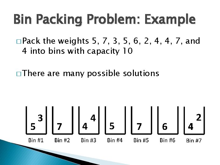
Bin Packing Problem: Example � Pack the weights 5, 7, 3, 5, 6, 2, 4, 4, 7, and 4 into bins with capacity 10 � There are many possible solutions

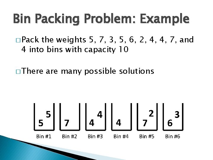
Bin Packing Problem: Example � Pack the weights 5, 7, 3, 5, 6, 2, 4, 4, 7, and 4 into bins with capacity 10 � There are many possible solutions

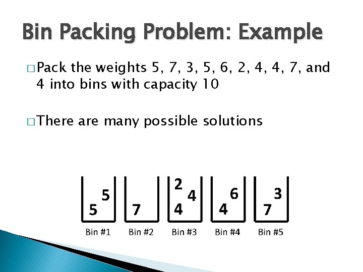
Bin Packing Problem: Example � Pack the weights 5, 7, 3, 5, 6, 2, 4, 4, 7, and 4 into bins with capacity 10 � There are many possible solutions

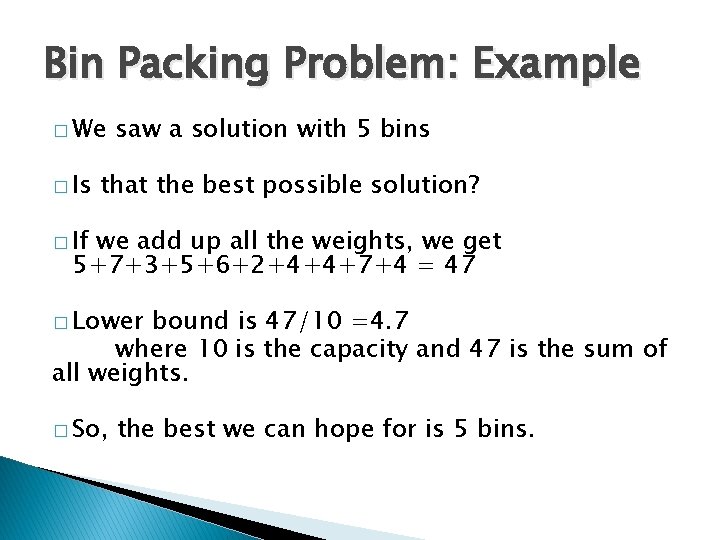
Bin Packing Problem: Example � We � Is saw a solution with 5 bins that the best possible solution? � If we add up all the weights, we get 5+7+3+5+6+2+4+4+7+4 = 47 � Lower bound is 47/10 =4. 7 where 10 is the capacity and 47 is the sum of all weights. � So, the best we can hope for is 5 bins.

Best Fit Decreasing Algorithm: Serial Approach � One heuristic method for packing weights is to look for these “best fits” � Consider all of the bins and find the bin that can hold the weight and would have the least room leftover after packing it. � One-at-a � We time algorithm have to decide what to do with each weight, in order, before moving on to the next one

Best Fit Decreasing Algorithm: Serial approach � Let’s start over and use the best fit decreasing algorithm � Sort the list of weights from the biggest to the smallest

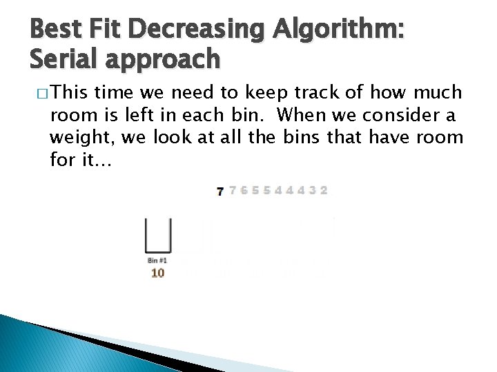
Best Fit Decreasing Algorithm: Serial approach � This time we need to keep track of how much room is left in each bin. When we consider a weight, we look at all the bins that have room for it…

Best Fit Decreasing Algorithm: Serial approach � …and put it into the bin that will have the least room left over � In this case, we only have one bin, so the 7 goes in there.

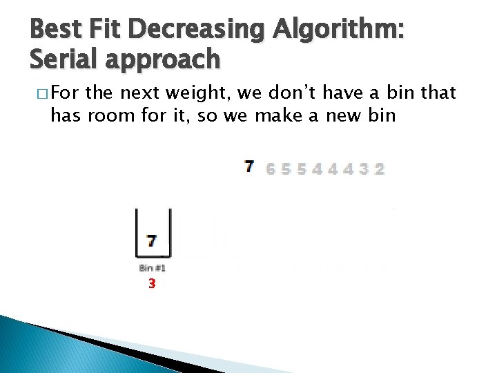
Best Fit Decreasing Algorithm: Serial approach � For the next weight, we don’t have a bin that has room for it, so we make a new bin 3

Best Fit Decreasing Algorithm: Serial approach � So, we make a new bin

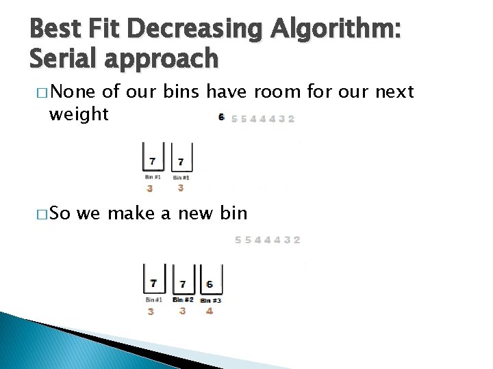
Best Fit Decreasing Algorithm: Serial approach � None of our bins have room for our next weight � So we make a new bin

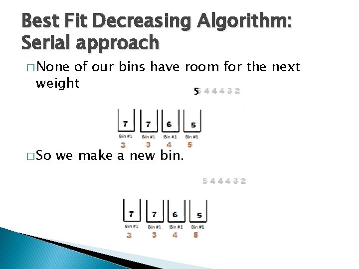
Best Fit Decreasing Algorithm: Serial approach � None of our bins have room for the next weight 5 � So we make a new bin.

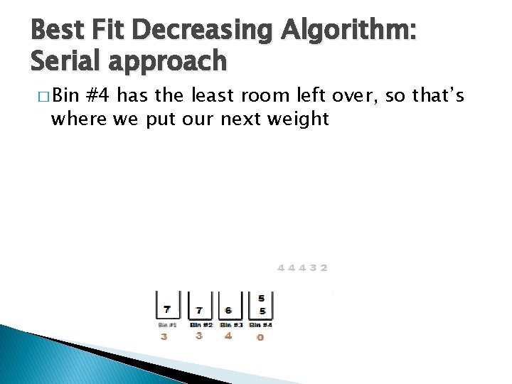
Best Fit Decreasing Algorithm: Serial approach � Bin #4 has the least room left over, so that’s where we put our next weight

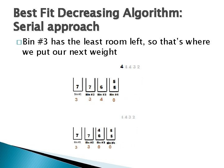
Best Fit Decreasing Algorithm: Serial approach � Bin #3 has the least room left, so that’s where we put our next weight

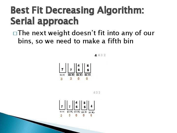
Best Fit Decreasing Algorithm: Serial approach � The next weight doesn’t fit into any of our bins, so we need to make a fifth bin

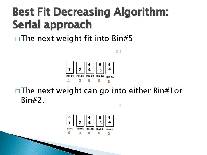
Best Fit Decreasing Algorithm: Serial approach � The next weight fit into Bin#5 next weight can go into either Bin#1 or Bin#2.

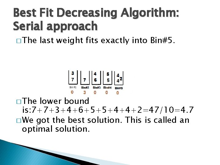
Best Fit Decreasing Algorithm: Serial approach � The last weight fits exactly into Bin#5. lower bound is: 7+7+3+4+6+5+5+4+4+2=47/10=4. 7 � We got the best solution. This is called an optimal solution.

Bin Packing Problem: Parallel Approach � If the list of weights is very long, or if the bin capacity is very large, this can be impractical. � The weights are tasks that need to be completed � The bins are “processors, ” which are the agents (people, machines, teams, etc. ) that will actually perform the tasks

Best Fit Decreasing Algorithm: Parallel Approach � Let’s start over and use the best decreasing fit algorithm in parallel implementation and using two cores with the same example. � Each core uses a bin. � The data set is divided into two parts with a cyclic data partition. � Each piece of data is mapped into a core (bin).

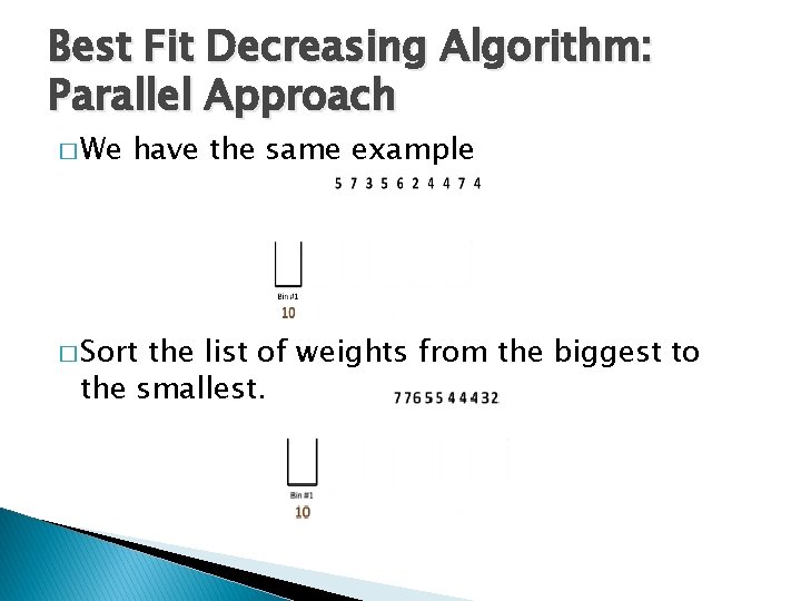
Best Fit Decreasing Algorithm: Parallel Approach � We have the same example � Sort the list of weights from the biggest to the smallest.

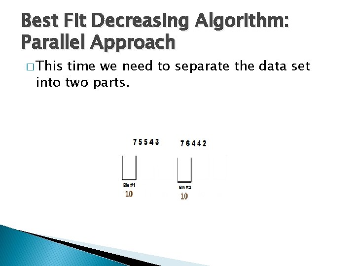
Best Fit Decreasing Algorithm: Parallel Approach � This time we need to separate the data set into two parts.

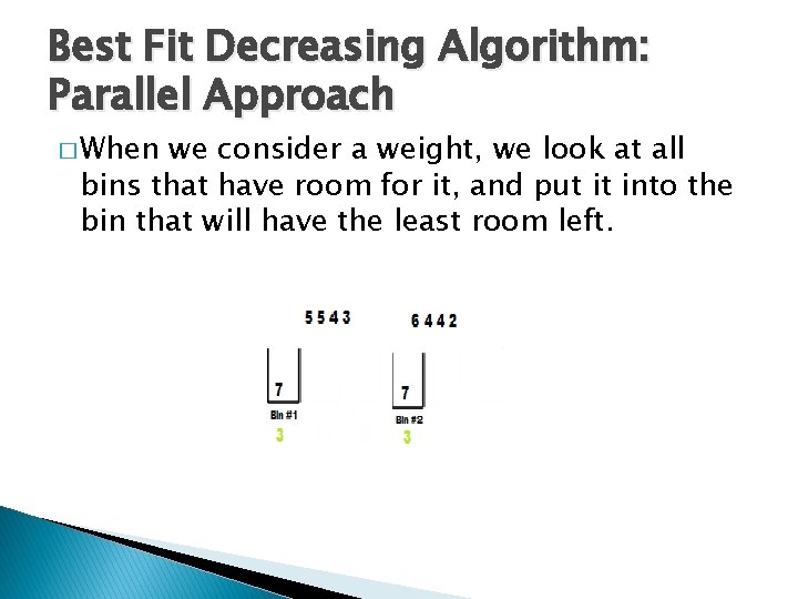
Best Fit Decreasing Algorithm: Parallel Approach � When we consider a weight, we look at all bins that have room for it, and put it into the bin that will have the least room left.

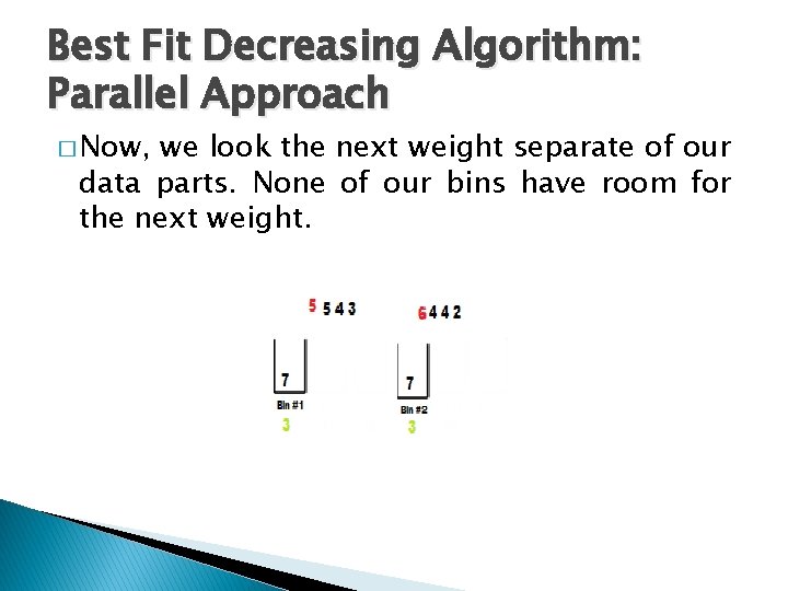
Best Fit Decreasing Algorithm: Parallel Approach � Now, we look the next weight separate of our data parts. None of our bins have room for the next weight.

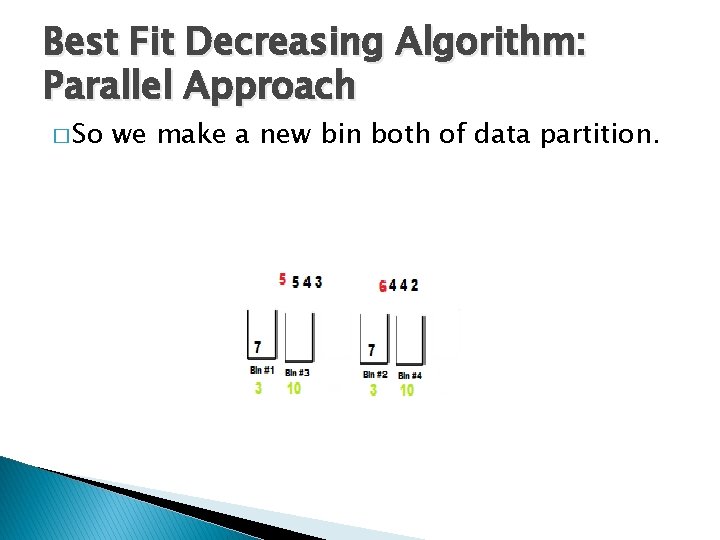
Best Fit Decreasing Algorithm: Parallel Approach � So we make a new bin both of data partition.

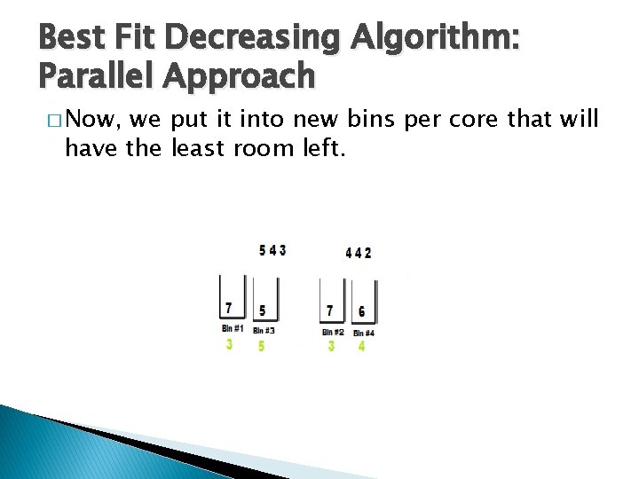
Best Fit Decreasing Algorithm: Parallel Approach � Now, we put it into new bins per core that will have the least room left.

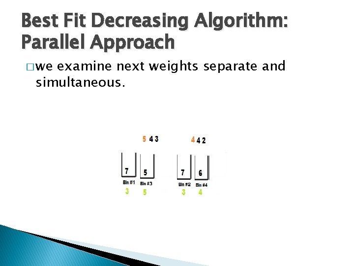
Best Fit Decreasing Algorithm: Parallel Approach � we examine next weights separate and simultaneous.

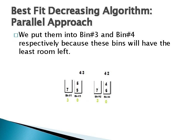
Best Fit Decreasing Algorithm: Parallel Approach � We put them into Bin#3 and Bin#4 respectively because these bins will have the least room left.

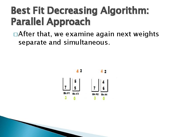
Best Fit Decreasing Algorithm: Parallel Approach � After that, we examine again next weights separate and simultaneous.

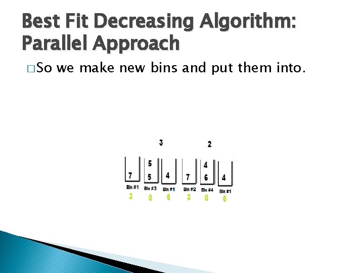
Best Fit Decreasing Algorithm: Parallel Approach � So we make new bins and put them into.

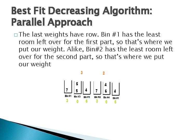
Best Fit Decreasing Algorithm: Parallel Approach � The last weights have row. Bin #1 has the least room left over for the first part, so that’s where we put our weight. Alike, Bin#2 has the least room left over for the second part, so that’s where we put our weight

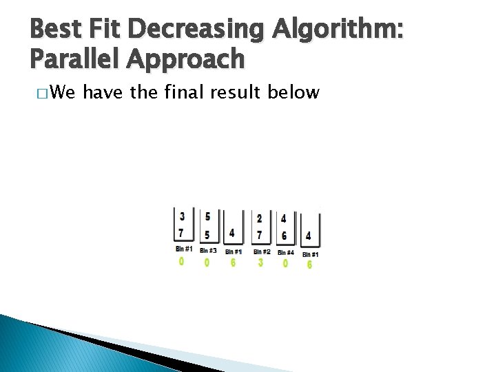
Best Fit Decreasing Algorithm: Parallel Approach � We have the final result below

Best Fit Decreasing Algorithm: Parallel Approach � This is a different result from the best fit decreasing algorithm. This is called also an optimal solution. The lower bound for the first part is 7+5+5+4+3=24/10=2. 4. Alike for the second part the lower bound is 7+6+4+4+2=23/10=2. 3. � We notice that the parallel implementation of algorithm use one more bin than serial, but it is executed in less steps.

Parallel vs Serial Approach � Will the serial execution of algorithm or the parallelization of algorithm be beneficial to us? From the previous examples, we can consider that: � For small datasets is preferable to use the serial algorithm. � For huge datasets is preferable to use the parallel algorithm.

Parallel vs Serial Approach � But, you should run the algorithm serial and then in parallel on different datasets. � In parallel execution, we will execute each dataset to varying number of processors in order to compare our results. � Only then, we say whether parallel processing is a beneficial or not.

Parallel Computing: Definations � Parallel computing is the use of multiple processors to execute different parts of the same program concurrently. �A parallel computer is a collection of processing elements, that can solve big problems quickly by means of well coordinated collaboration.

MATLAB- Parallel Computing Toolbox™ � The implementation and the execution of algorithms made in the laboratory "Parallel and Distributed Processing" at the premises of the department of Computer Engineering of the Technological educational institution of Central Macedonia. � For the run of Algorithm computers were used (total 32 Processors), each processor has a 2. 4 GHz. We used the software package MATLAB (version 6. 2).

MATLAB Computing Distributed Server To run applications in MATLAB Distributed Computing Server must be done the following steps: � Installation � Run � Set of the MDCE of MDCE up of the network with the admincenter

Installation and activation of MATLAB Computing Distributed Server � First, we set the current directory as MATLABR 2010 atoolboxdistcompbin � Afterwards, we run the in command window of MATLAB the following command !mdce install � Finally, we enable the MDCE in command window of MATLAB with the following command !mdce start

Set up of the network � We run the command admincenter outside of the MATLAB environment. � This commands occurs in directory � MATLABR 2010 atoolboxdistcompbin

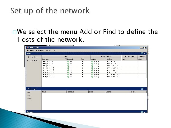
Set up of the network � We select the menu Add or Find to define the Hosts of the network.

Set up of the network � We create a Jobmanager by the menu Start in Jobmanager part, which is called “Bin. Packing. Man”. In this Job. Manager, we set up eight hostnames with 4 cores per hostname (PC).

Set up of the network � Close the admincenter window and we set by the menu parallel the Jobmanager.

MATLAB- Parallel Computing Toolbox™ � Parallel Computing Toolbox™ lets us solve computationally and data-intensive problems using multicore processors, GPUs, and computer clusters. � Totally, we had 32 cores. Then, we could run and executed Best Fit Decreasing algorithm parallel. We took the following useful conclusions on the execution time, the total wastage, the total number of bins used, the speed up and the efficiency on different size of datasets.

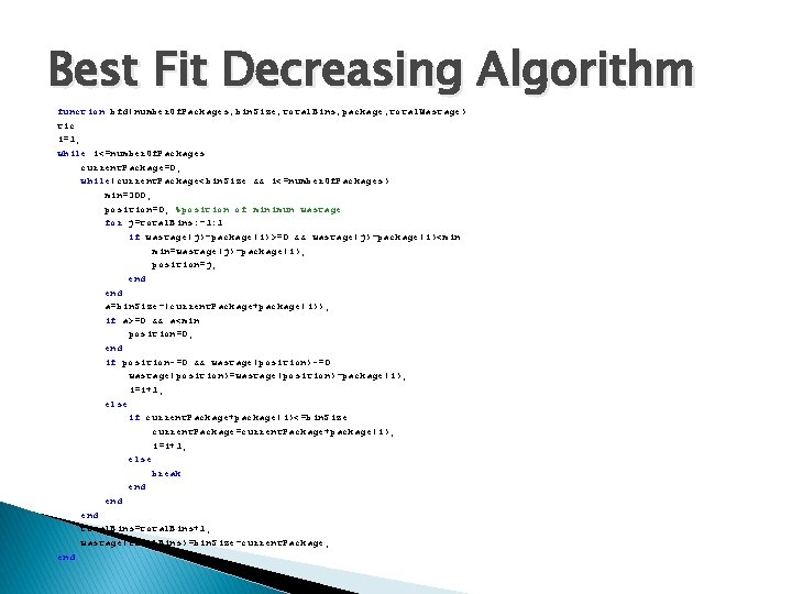
Best Fit Decreasing Algorithm function bfd(number. Of. Packages, bin. Size, total. Bins, package, total. Wastage) tic i=1; while i<=number. Of. Packages current. Package=0; while(current. Package<bin. Size && i<=number. Of. Packages) min=300; position=0; %position of minimun wastage for j=total. Bins: -1: 1 if wastage(j)-package(i)>=0 && wastage(j)-package(i)<min min=wastage(j)-package(i); position=j; end a=bin. Size-(current. Package+package(i)); if a>=0 && a<min position=0; end if position~=0 && wastage(position)~=0 wastage(position)=wastage(position)-package(i); i=i+1; else if current. Package+package(i)<=bin. Size current. Package=current. Package+package(i); i=i+1; else break end end total. Bins=total. Bins+1; wastage(total. Bins)=bin. Size-current. Package; end

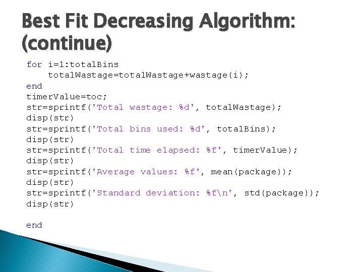
Best Fit Decreasing Algorithm: (continue) for i=1: total. Bins total. Wastage=total. Wastage+wastage(i); end timer. Value=toc; str=sprintf('Total wastage: %d', total. Wastage); disp(str) str=sprintf('Total bins used: %d', total. Bins); disp(str) str=sprintf('Total time elapsed: %f', timer. Value); disp(str) str=sprintf('Average values: %f', mean(package)); disp(str) str=sprintf('Standard deviation: %fn', std(package)); disp(str) end

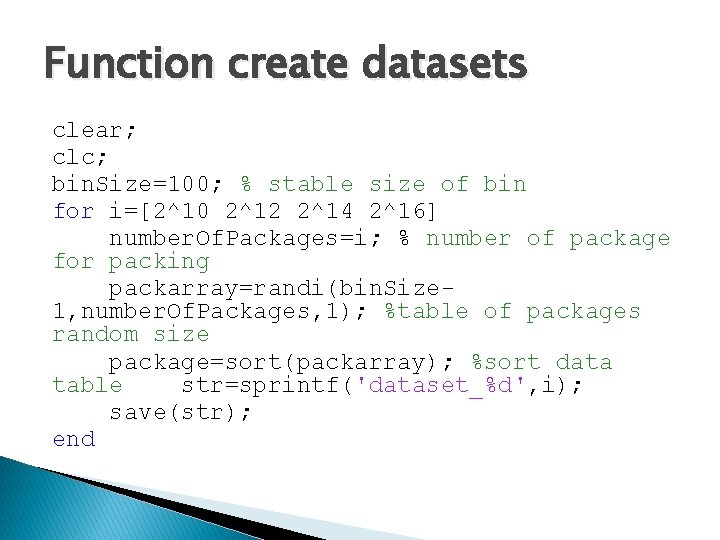
Function create datasets clear; clc; bin. Size=100; % stable size of bin for i=[2^10 2^12 2^14 2^16] number. Of. Packages=i; % number of package for packing packarray=randi(bin. Size 1, number. Of. Packages, 1); %table of packages random size package=sort(packarray); %sort data table str=sprintf('dataset_%d', i); save(str); end

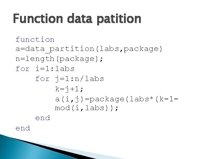
Function data patition function a=data_partition(labs, package) n=length(package); for i=1: labs for j=1: n/labs k=j+1; a(i, j)=package(labs*(k-1 mod(i, labs)); end

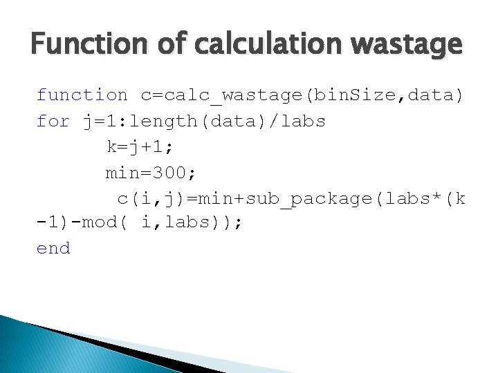
Function of calculation wastage function c=calc_wastage(bin. Size, data) for j=1: length(data)/labs k=j+1; min=300; c(i, j)=min+sub_package(labs*(k -1)-mod( i, labs)); end

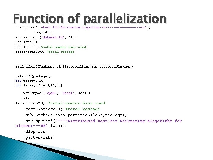
Function of parallelization str=sprintf('-Best Fit Decreasing Algorithm-n---------n' ); disp(str); str 1=sprintf('dataset_%d', 2^10); load(str 1); total. Bins=0; %total number bins used total. Wastage=0; %total wastage bfd(number. Of. Packages, bin. Size, total. Bins, package, total. Wastage ) n=length(package); for tloop=1: 10 for labs=[1, 2, 4, 8, 16, 32] matlabpool('open', 'local', labs); tic total. Bins=0; %total number bins used total. Wastage=0; %total wastage sub_package=data_partition(labs, package); str=sprintf('----Distributed Best Fit Decreasing Alogorithm for clones: ---%d', labs); disp(str) part=n/labs;

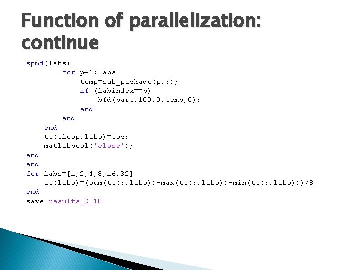
Function of parallelization: continue spmd(labs) for p=1: labs temp=sub_package(p, : ); if (labindex==p) bfd(part, 100, 0, temp, 0); end end tt(tloop, labs)=toc; matlabpool('close'); end for labs=[1, 2, 4, 8, 16, 32] at(labs)=(sum(tt(: , labs))-max(tt(: , labs))-min(tt(: , labs)))/8 end save results_2_10

Explanation of Code The command matlabpool enables the parallel language features in the MATLAB language by starting a parallel job that connects this MATLAB client with a number of labs. matlabpool('open', 'local', labs); starts a worker pool using the local parallel configuration and the number of the available labs is labs. matlabpool('close'); stops the worker pool, destroys the parallel job, and makes all parallel language features revert to using the MATLAB client for computing their results.

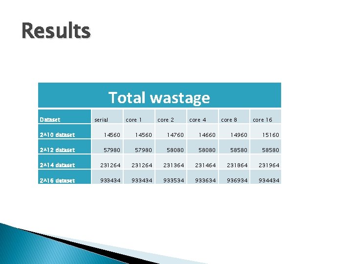
Results Total wastage Dataset serial core 1 core 2 core 4 core 8 core 16 2^10 dataset 14560 14760 14660 14960 15160 2^12 dataset 57980 58080 58580 2^14 dataset 231264 231364 231464 231864 231964 2^16 dataset 933434 933534 933634 936934 934434

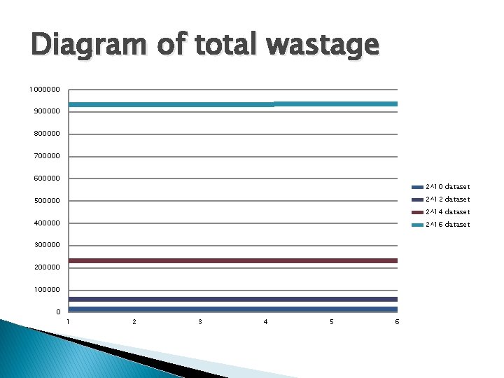
Diagram of total wastage 1000000 900000 800000 700000 600000 2^10 dataset 2^12 dataset 500000 2^14 dataset 400000 2^16 dataset 300000 200000 100000 0 1 2 3 4 5 6

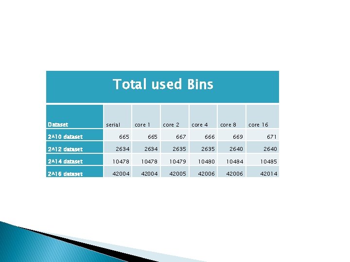
Total used Bins Dataset serial core 1 core 2 core 4 core 8 core 16 2^10 dataset 665 667 666 669 671 2^12 dataset 2634 2635 2640 2^14 dataset 10478 10479 10480 10484 10485 2^16 dataset 42004 42005 42006 42014

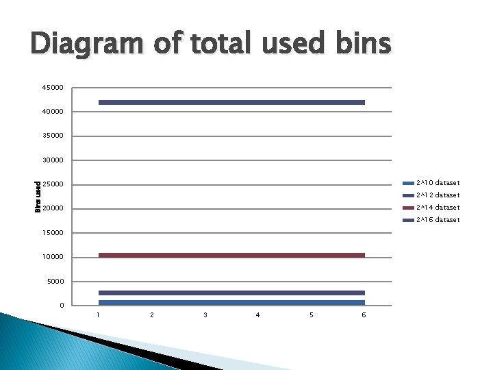
Diagram of total used bins 45000 40000 35000 30000 2^10 dataset Bins used 25000 2^12 dataset 2^14 dataset 20000 2^16 dataset 15000 10000 5000 0 1 2 3 4 5 6

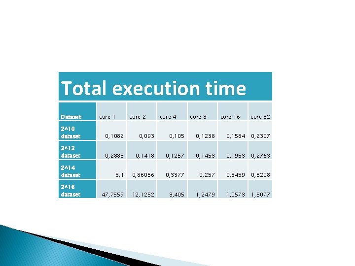
Total execution time Dataset core 1 core 2 core 4 core 8 core 16 core 32 2^10 dataset 0, 1082 0, 093 0, 105 0, 1238 0, 1584 0, 2307 2^12 dataset 0, 2883 0, 1418 0, 1257 0, 1453 0, 1953 0, 2763 2^14 dataset 3, 1 0, 86056 0, 3377 0, 257 0, 3459 0, 5208 2^16 dataset 47, 7559 12, 1252 3, 405 1, 2479 1, 0573 1, 5077

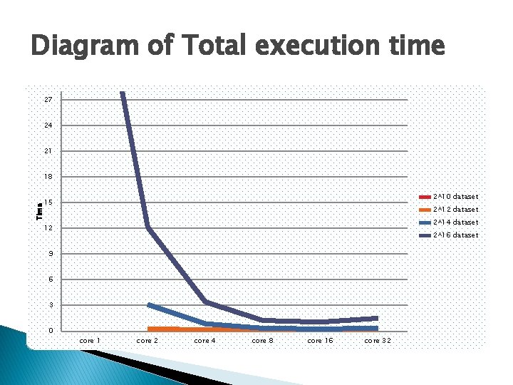
Diagram of Total execution time 27 24 21 18 2^10 dataset Time 15 2^12 dataset 2^14 dataset 12 2^16 dataset 9 6 3 0 core 1 core 2 core 4 core 8 core 16 core 32

Thank you!