Bilkent University Department of Computer Engineering CS 342

Bilkent University Department of Computer Engineering CS 342 Operating Systems Chapter 5 Process Scheduling Dr. Selim Aksoy http: //www. cs. bilkent. edu. tr/~saksoy Slides courtesy of Dr. İbrahim Körpeoğlu 1

Objectives and Outline • Basic Concepts • Scheduling Criteria • Scheduling Algorithms • Thread Scheduling • Multiple-Processor Scheduling • Operating Systems Examples • Algorithm Evaluation Objective • To introduce CPU scheduling, which is the basis for multiprogrammed operating systems • To describe various CPUscheduling algorithms • To discuss evaluation criteria for selecting a CPU-scheduling algorithm for a particular system 2

Basic Concepts • Maximum CPU utilization obtained with multiprogramming • CPU–I/O Burst Cycle – Process execution consists of a cycle of CPU execution and I/O wait • CPU burst distribution 3

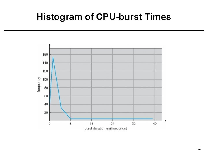
Histogram of CPU-burst Times 4

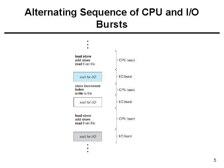
Alternating Sequence of CPU and I/O Bursts 5

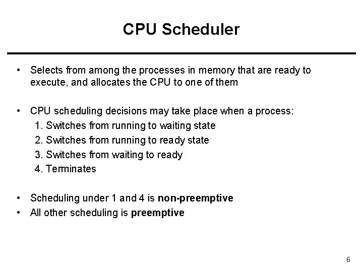
CPU Scheduler • Selects from among the processes in memory that are ready to execute, and allocates the CPU to one of them • CPU scheduling decisions may take place when a process: 1. Switches from running to waiting state 2. Switches from running to ready state 3. Switches from waiting to ready 4. Terminates • Scheduling under 1 and 4 is non-preemptive • All other scheduling is preemptive 6

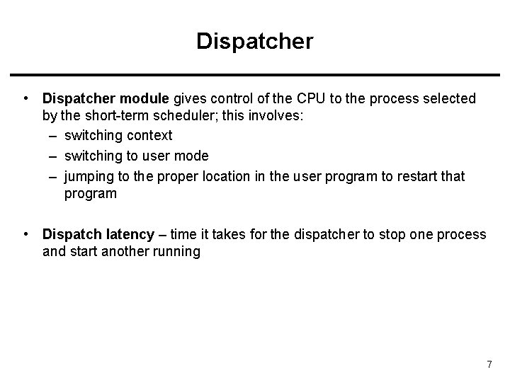
Dispatcher • Dispatcher module gives control of the CPU to the process selected by the short-term scheduler; this involves: – switching context – switching to user mode – jumping to the proper location in the user program to restart that program • Dispatch latency – time it takes for the dispatcher to stop one process and start another running 7

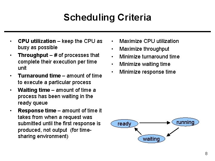
Scheduling Criteria • • • CPU utilization – keep the CPU as busy as possible Throughput – # of processes that complete their execution per time unit Turnaround time – amount of time to execute a particular process Waiting time – amount of time a process has been waiting in the ready queue Response time – amount of time it takes from when a request was submitted until the first response is produced, not output (for timesharing environment) • • • Maximize CPU utilization Maximize throughput Minimize turnaround time Minimize waiting time Minimize response time running ready waiting 8

Some Scheduling Algorithms 9

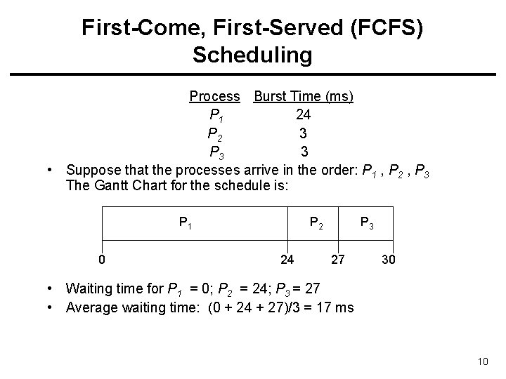
First-Come, First-Served (FCFS) Scheduling Process Burst Time (ms) P 1 24 P 2 3 P 3 3 • Suppose that the processes arrive in the order: P 1 , P 2 , P 3 The Gantt Chart for the schedule is: P 1 0 P 2 24 P 3 27 30 • Waiting time for P 1 = 0; P 2 = 24; P 3 = 27 • Average waiting time: (0 + 24 + 27)/3 = 17 ms 10

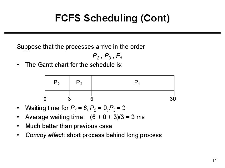
FCFS Scheduling (Cont) Suppose that the processes arrive in the order P 2 , P 3 , P 1 • The Gantt chart for the schedule is: P 2 0 • • P 3 3 P 1 6 30 Waiting time for P 1 = 6; P 2 = 0; P 3 = 3 Average waiting time: (6 + 0 + 3)/3 = 3 ms Much better than previous case Convoy effect: short process behind long process 11

Shortest-Job-First (SJF) Scheduling • Associate with each process the length of its next CPU burst. Use these lengths to schedule the process with the shortest time • SJF is optimal – gives minimum average waiting time for a given set of processes – The difficulty is knowing the length of the next CPU request 12

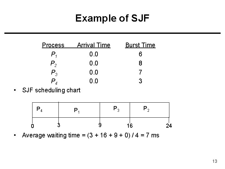
Example of SJF Process Arrival Time P 1 0. 0 P 2 0. 0 P 3 0. 0 P 4 0. 0 • SJF scheduling chart P 4 0 P 3 P 1 3 Burst Time 6 8 7 3 9 P 2 16 24 • Average waiting time = (3 + 16 + 9 + 0) / 4 = 7 ms 13

Determining Length of Next CPU Burst • Can only estimate the length • Can be done by using the length of previous CPU bursts, using exponential averaging 14

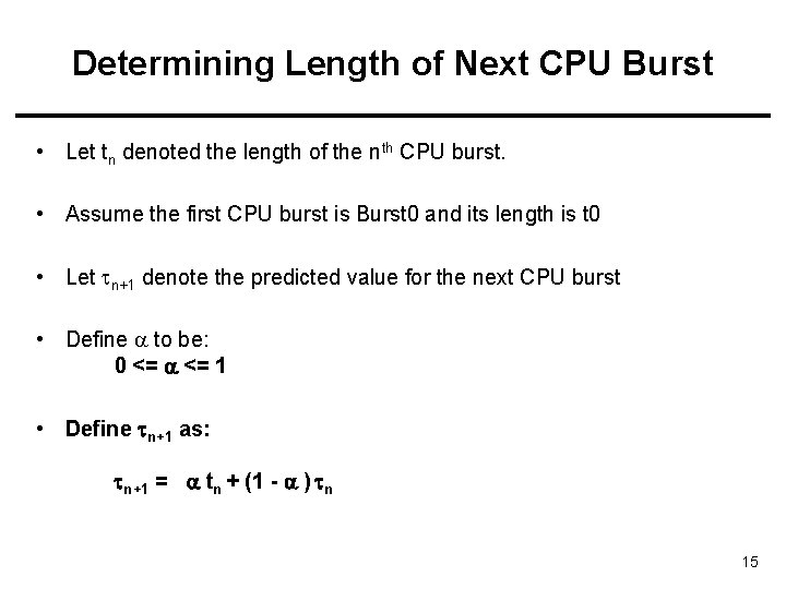
Determining Length of Next CPU Burst • Let tn denoted the length of the nth CPU burst. • Assume the first CPU burst is Burst 0 and its length is t 0 • Let n+1 denote the predicted value for the next CPU burst • Define to be: 0 <= 1 • Define n+1 as: n+1 = tn + (1 - ) n 15

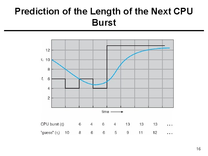
Prediction of the Length of the Next CPU Burst 16

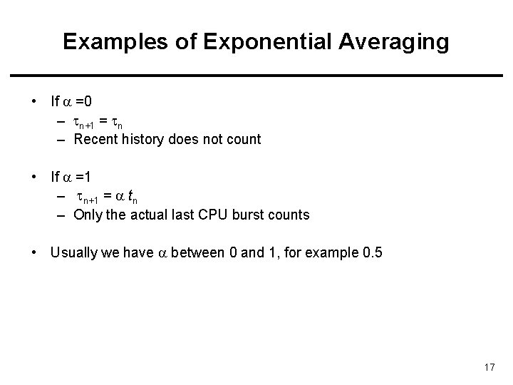
Examples of Exponential Averaging • If =0 – n+1 = n – Recent history does not count • If =1 – n+1 = tn – Only the actual last CPU burst counts • Usually we have between 0 and 1, for example 0. 5 17

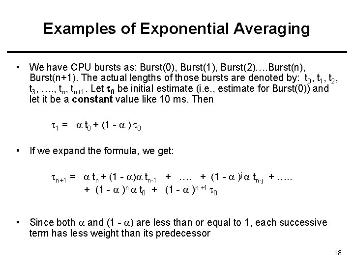
Examples of Exponential Averaging • We have CPU bursts as: Burst(0), Burst(1), Burst(2)…. Burst(n), Burst(n+1). The actual lengths of those bursts are denoted by: t 0, t 1, t 2, t 3, …. , tn+1. Let 0 be initial estimate (i. e. , estimate for Burst(0)) and let it be a constant value like 10 ms. Then 1 = t 0 + (1 - ) 0 • If we expand the formula, we get: n+1 = tn + (1 - ) tn-1 + …. + (1 - )j tn-j + …. . + (1 - )n t 0 + (1 - )n +1 0 • Since both and (1 - ) are less than or equal to 1, each successive term has less weight than its predecessor 18

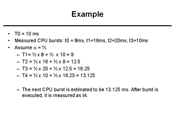
Example • T 0 = 10 ms • Measured CPU bursts: t 0 = 8 ms, t 1=16 ms, t 2=20 ms, t 3=10 ms • Assume = ½ – T 1= ½ x 8 + ½ x 10 = 9 – T 2 = ½ x 16 + ½ x 9 = 12. 5 – T 3 = ½ x 20 + ½ x 12. 5 = 16. 25 – T 4 = ½ x 10 + ½ x 16. 25 = 13. 125 – The next CPU burst is estimated to be 13. 125 ms. After burst is executed, it is measured as t 4.

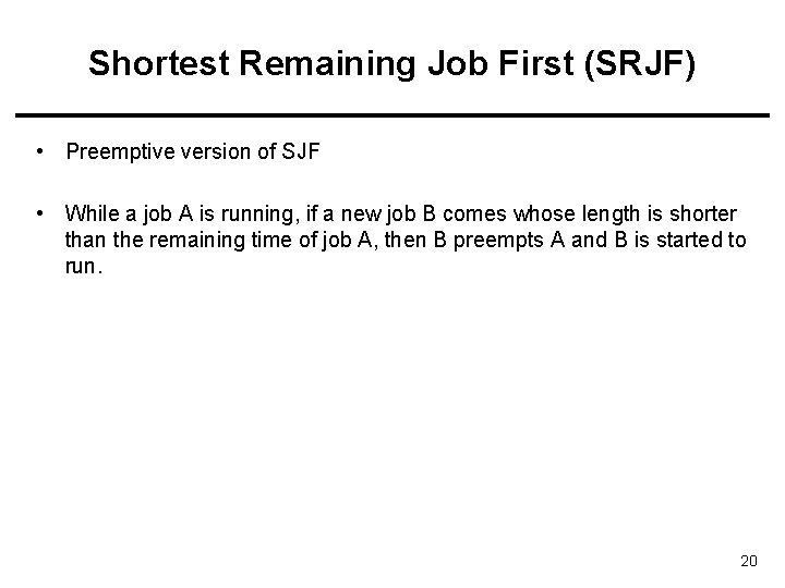
Shortest Remaining Job First (SRJF) • Preemptive version of SJF • While a job A is running, if a new job B comes whose length is shorter than the remaining time of job A, then B preempts A and B is started to run. 20

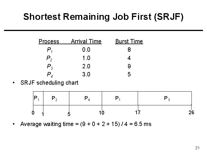
Shortest Remaining Job First (SRJF) Process Arrival Time P 1 0. 0 P 2 1. 0 P 3 2. 0 P 4 3. 0 • SRJF scheduling chart P 1 0 P 2 1 P 4 5 Burst Time 8 4 9 5 P 1 10 P 3 17 26 • Average waiting time = (9 + 0 + 2 + 15) / 4 = 6. 5 ms 21

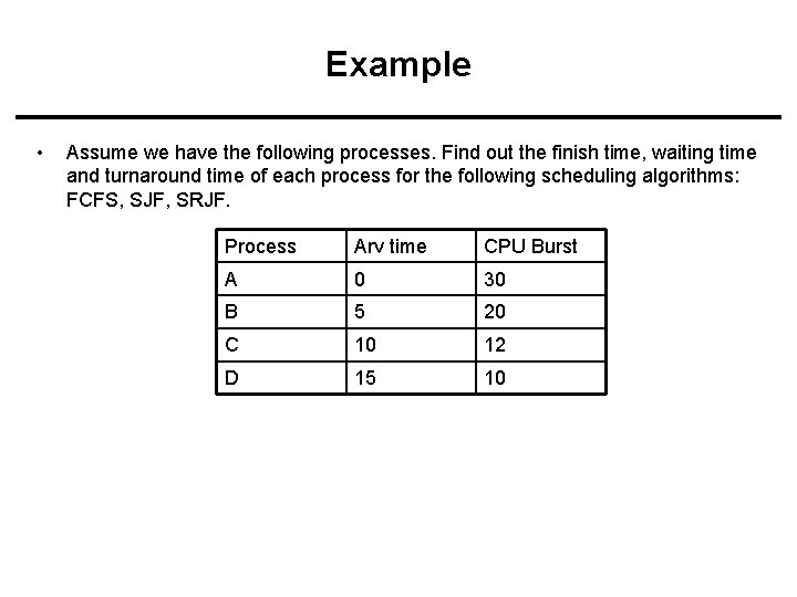
Example • Assume we have the following processes. Find out the finish time, waiting time and turnaround time of each process for the following scheduling algorithms: FCFS, SJF, SRJF. Process Arv time CPU Burst A 0 30 B 5 20 C 10 12 D 15 10

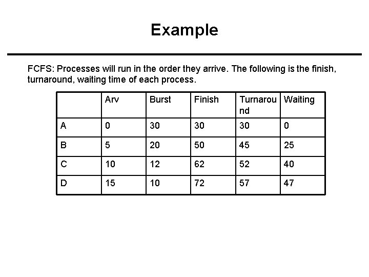
Example FCFS: Processes will run in the order they arrive. The following is the finish, turnaround, waiting time of each process. Arv Burst Finish Turnarou Waiting nd A 0 30 30 30 0 B 5 20 50 45 25 C 10 12 62 52 40 D 15 10 72 57 47

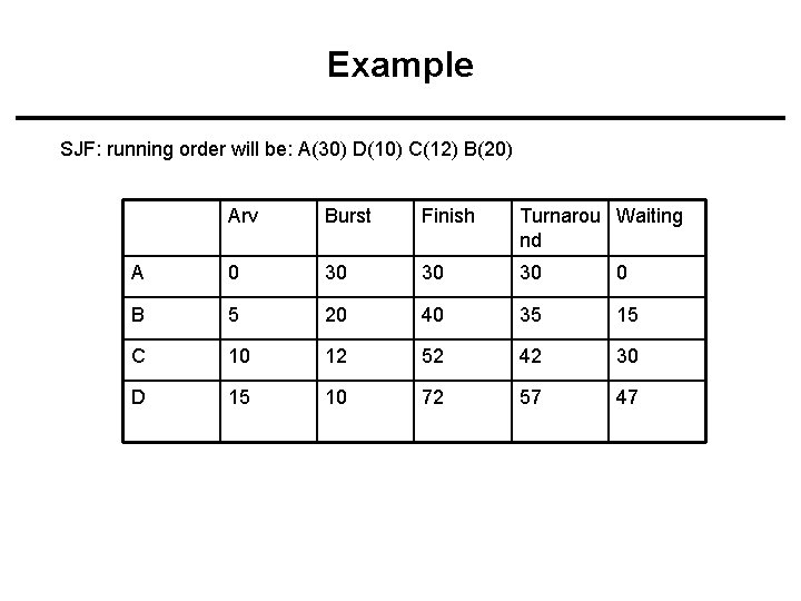
Example SJF: running order will be: A(30) D(10) C(12) B(20) Arv Burst Finish Turnarou Waiting nd A 0 30 30 30 0 B 5 20 40 35 15 C 10 12 52 42 30 D 15 10 72 57 47

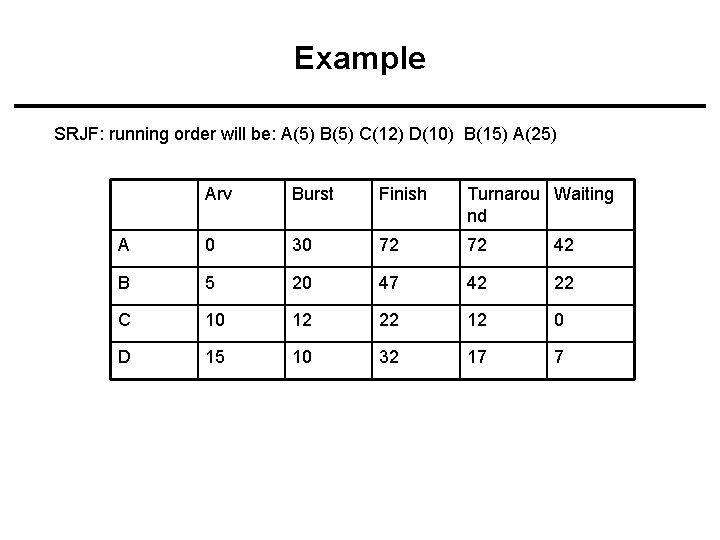
Example SRJF: running order will be: A(5) B(5) C(12) D(10) B(15) A(25) Arv Burst Finish Turnarou Waiting nd A 0 30 72 72 42 B 5 20 47 42 22 C 10 12 22 12 0 D 15 10 32 17 7

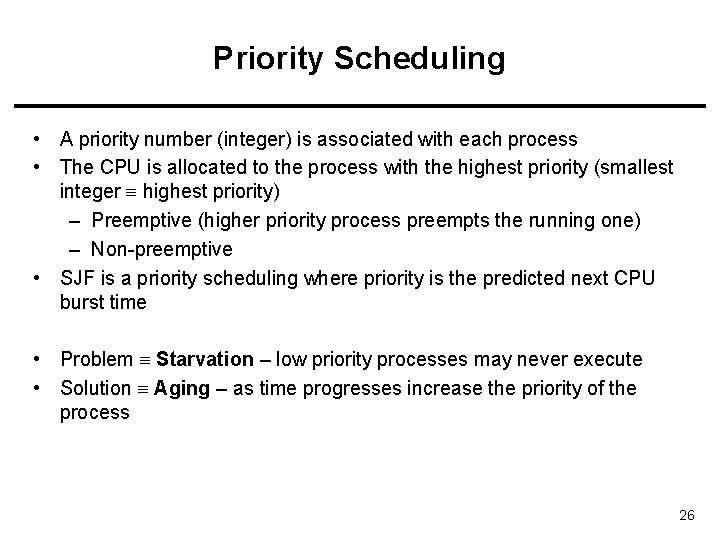
Priority Scheduling • A priority number (integer) is associated with each process • The CPU is allocated to the process with the highest priority (smallest integer highest priority) – Preemptive (higher priority process preempts the running one) – Non-preemptive • SJF is a priority scheduling where priority is the predicted next CPU burst time • Problem Starvation – low priority processes may never execute • Solution Aging – as time progresses increase the priority of the process 26

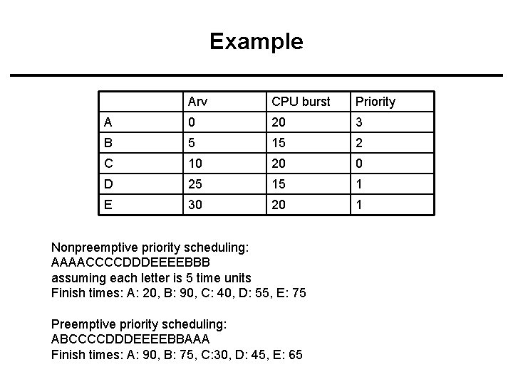
Example Arv CPU burst Priority A 0 20 3 B 5 15 2 C 10 20 0 D 25 15 1 E 30 20 1 Nonpreemptive priority scheduling: AAAACCCCDDDEEEEBBB assuming each letter is 5 time units Finish times: A: 20, B: 90, C: 40, D: 55, E: 75 Preemptive priority scheduling: ABCCCCDDDEEEEBBAAA Finish times: A: 90, B: 75, C: 30, D: 45, E: 65

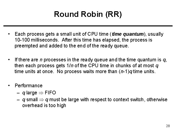
Round Robin (RR) • Each process gets a small unit of CPU time (time quantum), usually 10 -100 milliseconds. After this time has elapsed, the process is preempted and added to the end of the ready queue. • If there are n processes in the ready queue and the time quantum is q, then each process gets 1/n of the CPU time in chunks of at most q time units at once. No process waits more than (n-1)q time units. • Performance – q large FIFO – q small q must be large with respect to context switch, otherwise overhead is too high 28

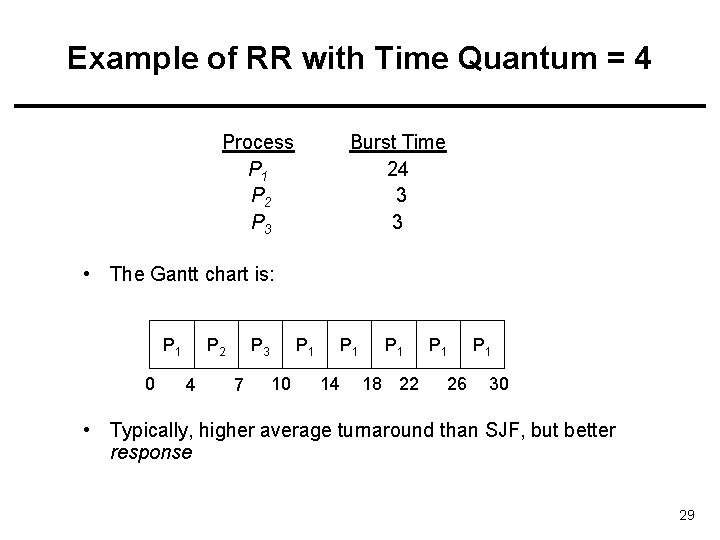
Example of RR with Time Quantum = 4 Process P 1 P 2 P 3 Burst Time 24 3 3 • The Gantt chart is: P 1 0 P 2 4 P 3 7 P 1 10 P 1 14 P 1 18 22 P 1 26 P 1 30 • Typically, higher average turnaround than SJF, but better response 29

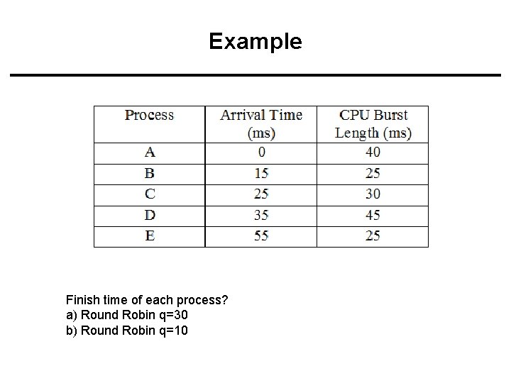
Example Finish time of each process? a) Round Robin q=30 b) Round Robin q=10

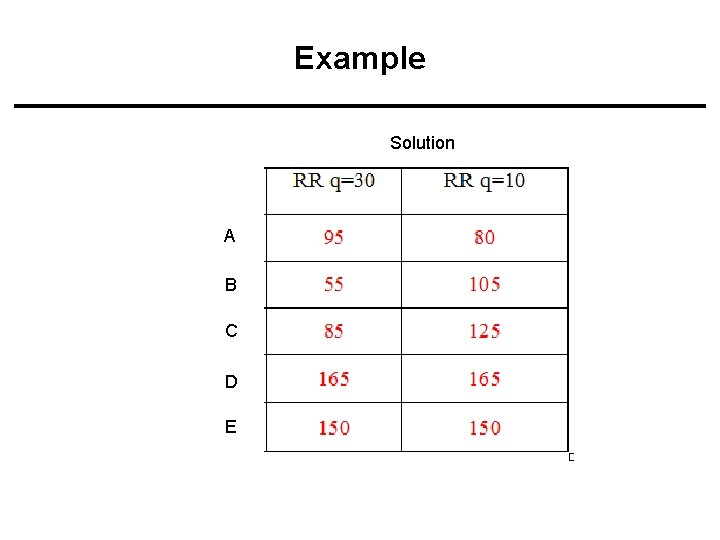
Example Solution A B C D E

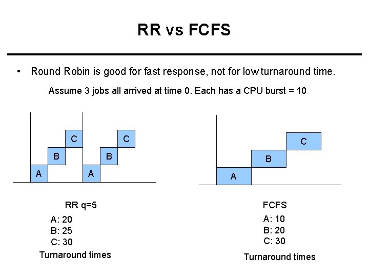
RR vs FCFS • Round Robin is good for fast response, not for low turnaround time. Assume 3 jobs all arrived at time 0. Each has a CPU burst = 10 C C B A RR q=5 A: 20 B: 25 C: 30 Turnaround times B A FCFS A: 10 B: 20 C: 30 Turnaround times

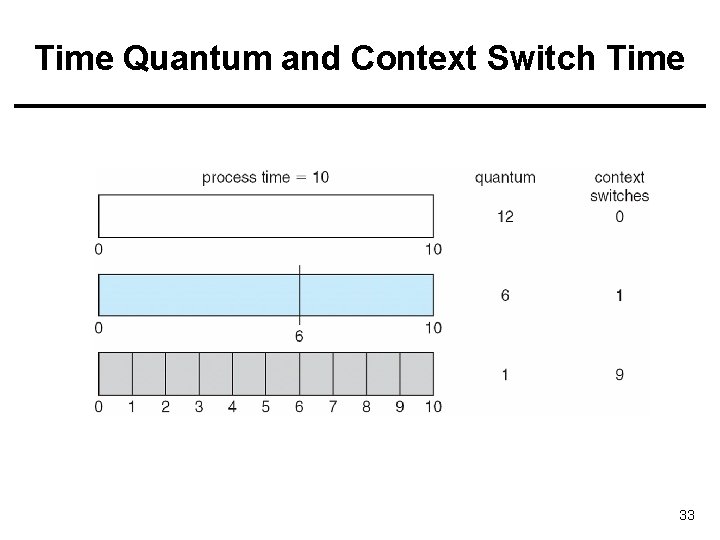
Time Quantum and Context Switch Time 33

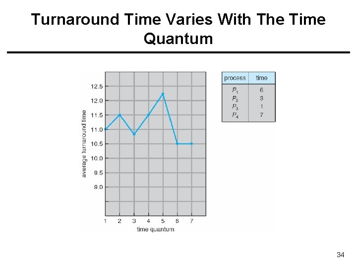
Turnaround Time Varies With The Time Quantum 34

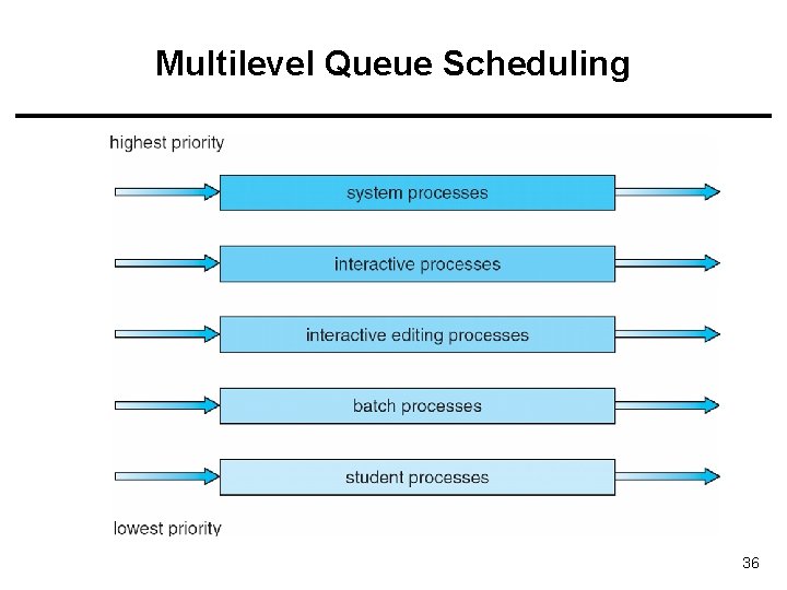
Multilevel Queue • Ready queue is partitioned into separate queues: foreground (interactive) background (batch) • Each queue has its own scheduling algorithm – foreground – RR – background – FCFS • Scheduling must be done between the queues – Fixed priority scheduling; (i. e. , serve all from foreground then from background). Possibility of starvation. – Time slice – each queue gets a certain amount of CPU time which it can schedule amongst its processes; i. e. , 80% to foreground in RR; 20% to background in FCFS 35

Multilevel Queue Scheduling 36

Multilevel Feedback Queue • A process can move between the various queues; aging can be implemented this way • Multilevel-feedback-queue scheduler defined by the following parameters: – number of queues – scheduling algorithms for each queue – method used to determine when to upgrade a process – method used to determine when to demote a process – method used to determine which queue a process will enter when that process needs service 37

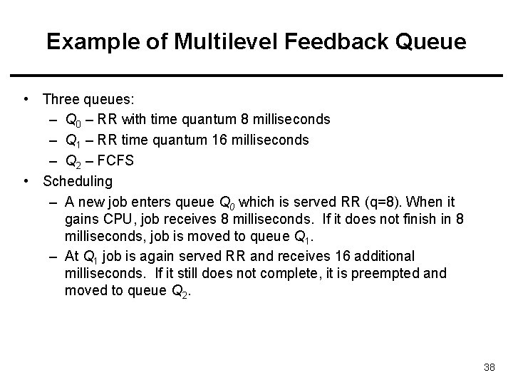
Example of Multilevel Feedback Queue • Three queues: – Q 0 – RR with time quantum 8 milliseconds – Q 1 – RR time quantum 16 milliseconds – Q 2 – FCFS • Scheduling – A new job enters queue Q 0 which is served RR (q=8). When it gains CPU, job receives 8 milliseconds. If it does not finish in 8 milliseconds, job is moved to queue Q 1. – At Q 1 job is again served RR and receives 16 additional milliseconds. If it still does not complete, it is preempted and moved to queue Q 2. 38

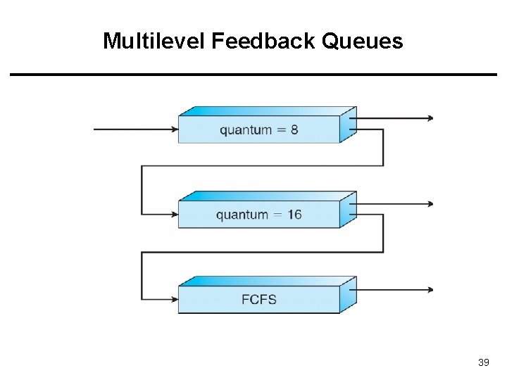
Multilevel Feedback Queues 39

Thread Scheduling 40

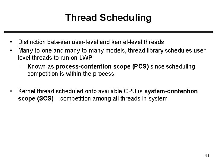
Thread Scheduling • Distinction between user-level and kernel-level threads • Many-to-one and many-to-many models, thread library schedules userlevel threads to run on LWP – Known as process-contention scope (PCS) since scheduling competition is within the process • Kernel thread scheduled onto available CPU is system-contention scope (SCS) – competition among all threads in system 41

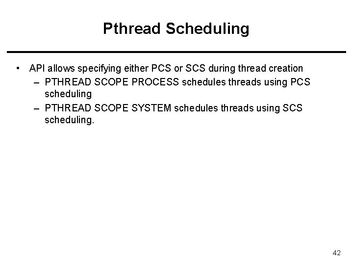
Pthread Scheduling • API allows specifying either PCS or SCS during thread creation – PTHREAD SCOPE PROCESS schedules threads using PCS scheduling – PTHREAD SCOPE SYSTEM schedules threads using SCS scheduling. 42

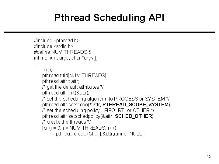
Pthread Scheduling API #include <pthread. h> #include <stdio. h> #define NUM THREADS 5 int main(int argc, char *argv[]) { int i; pthread t tid[NUM THREADS]; pthread attr t attr; /* get the default attributes */ pthread attr init(&attr); /* set the scheduling algorithm to PROCESS or SYSTEM */ pthread attr setscope(&attr, PTHREAD_SCOPE_SYSTEM); /* set the scheduling policy - FIFO, RT, or OTHER */ pthread attr setschedpolicy(&attr, SCHED_OTHER); /* create threads */ for (i = 0; i < NUM THREADS; i++) pthread create(&tid[i], &attr, runner, NULL); 43

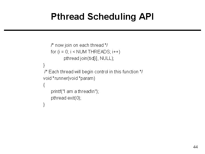
Pthread Scheduling API /* now join on each thread */ for (i = 0; i < NUM THREADS; i++) pthread join(tid[i], NULL); } /* Each thread will begin control in this function */ void *runner(void *param) { printf("I am a threadn"); pthread exit(0); } 44

Multiprocessor Scheduling 45

Multiple-Processor Scheduling • CPU scheduling more complex when multiple CPUs are available • Homogeneous processors within a multiprocessor • Asymmetric multiprocessing – only one processor accesses the system data structures, alleviating the need for data sharing • Symmetric multiprocessing (SMP) – each processor is selfscheduling, all processes in common ready queue, or each has its own private queue of ready processes • Processor affinity – process has affinity for processor on which it is currently running – soft affinity – hard affinity 46

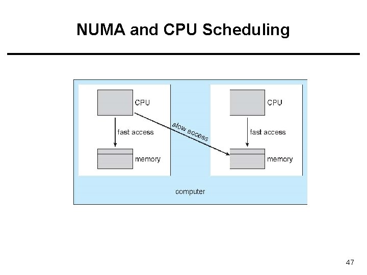
NUMA and CPU Scheduling 47

Multicore Processors • Recent trend to place multiple processor cores on same physical chip • Faster and consume less power • Multiple threads per core also growing – Takes advantage of memory stall to make progress on another thread while memory retrieve happens 48

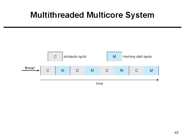
Multithreaded Multicore System 49

Examples from Operating Systems 50

Operating System Examples • Solaris scheduling • Windows XP scheduling • Linux scheduling 51

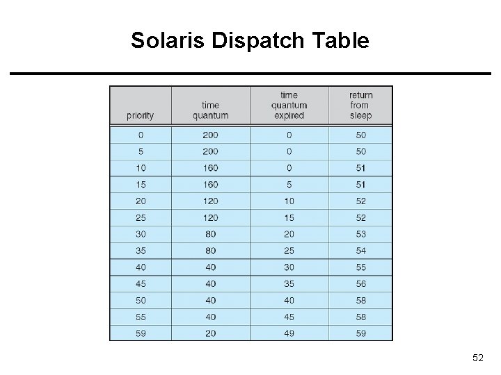
Solaris Dispatch Table 52

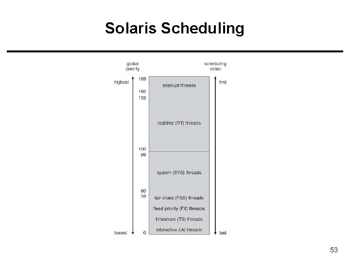
Solaris Scheduling 53

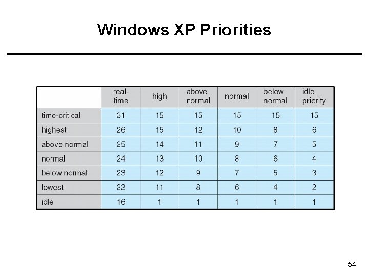
Windows XP Priorities 54

Linux Scheduling • • Constant order O(1) scheduling time Two priority ranges: time-sharing and real-time Real-time range from 0 to 99 and nice value from 100 to 140 (figure 5. 15) 55

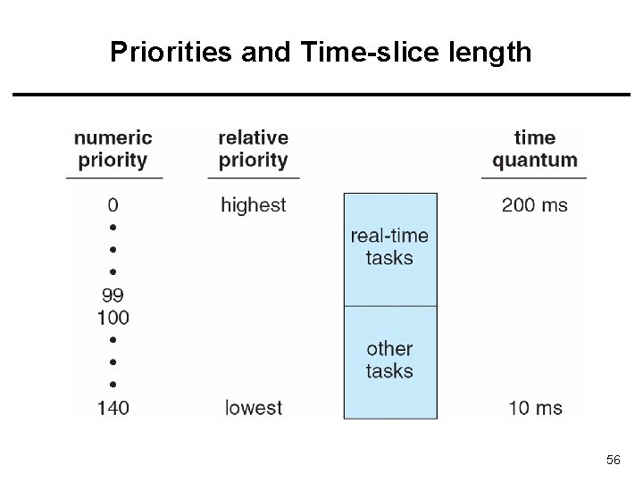
Priorities and Time-slice length 56

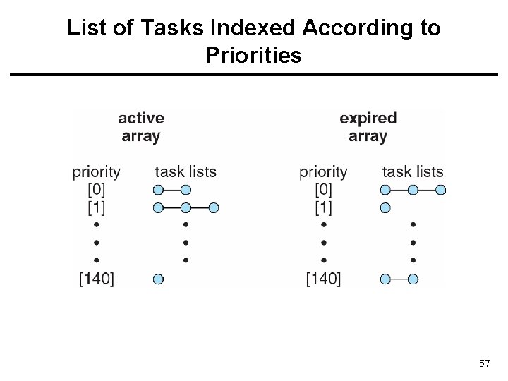
List of Tasks Indexed According to Priorities 57

Algorithm Evaluation 58

Algorithm Evaluation • Deterministic modeling – takes a particular predetermined workload and defines the performance of each algorithm for that workload – One form of analytic evaluation – Valid for a particular scenario and input. • Queuing models • Simulation • Implementation 59

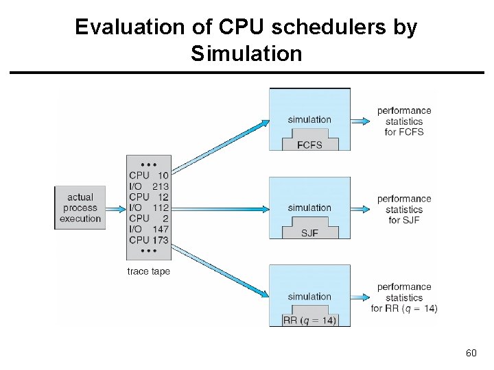
Evaluation of CPU schedulers by Simulation 60

References • The slides here adapted/modified from the textbook and its slides: Operating System Concepts, Silberschatz et al. , 7 th & 8 th editions, Wiley. • Operating System Concepts, 7 th and 8 th editions, Silberschatz et al. Wiley. • Modern Operating Systems, Andrew S. Tanenbaum, 3 rd edition, 2009 61