Bilinear Classifiers for Visual Recognition Hamed Pirsiavash Deva

Bilinear Classifiers for Visual Recognition Hamed Pirsiavash Deva Ramanan Charless Fowlkes Computational Vision Lab. University of California Irvine To be presented in NIPS 2009 1

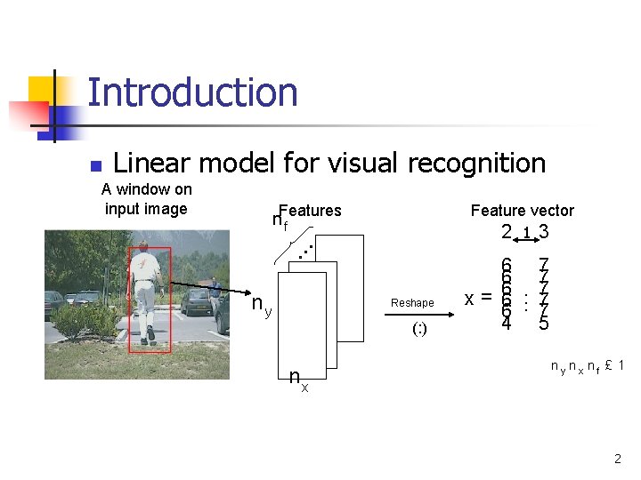
Introduction n Linear model for visual recognition A window on input image n. Features f ny Feature vector 2 13 Reshape (: ) nx 6 7 6 7 x = 6. . . 7 6 7 4 5 ny nx nf £ 1 2

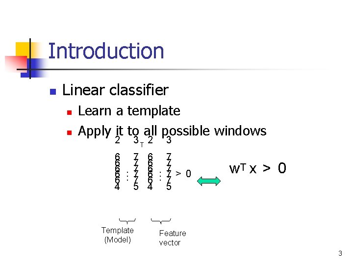
Introduction n Linear classifier n n Learn a template Apply it to all possible windows 2 3 T 2 3 6 7 6 7 6. 7> 0 6 7 4 5 Template (Model) w. T x > 0 Feature vector 3

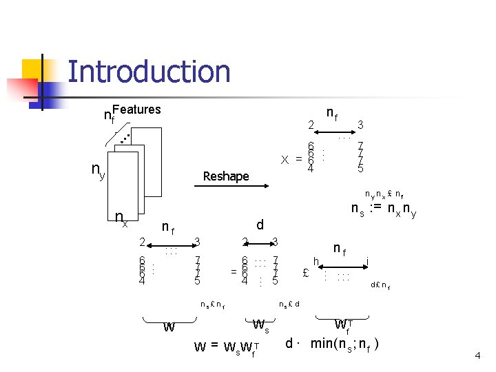
Introduction nf. Features nf 2 ny 6. . 6 X = 6. 4 Reshape 3 : : : 7 7 7 5 ny nx £ nf nx 2 6. 6 4 nf : : : d 3 2 7 7 7 5 3 6 : : : 7 7 = 6 6. . 7 4. 5 ns£ nf W n s : = n x n y £ h nf. . . : : : i d£ n f ns £ d Ws W = Ws W T f WT f d · min(n s ; n f ) 4

Introduction n Motivation for bilinear models n Reduced rank: less number of parameters n n n Better generalization: reduced over-fitting Run-time efficiency Transfer learning n Share a subset of parameters between different but related tasks 5

Outline n n n Introduction Sliding window classifiers Bilinear model and its motivation Extension Related work Experiments n n n Pedestrian detection Human action classification Conclusion 6

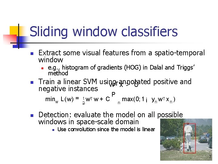
Sliding window classifiers n Extract some visual features from a spatio-temporal window n n e. g. , histogram of gradients (HOG) in Dalal and Triggs’ method Train a linear SVM using positive and w T annotated x> 0 negative instances minw L (w) = n 1 w. T w 2 + C P n max(0; 1 ¡ yn w. T x n ) Detection: evaluate the model on all possible windows in space-scale domain n Use convolution since the model is linear 7

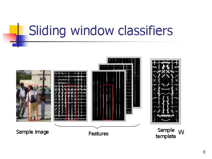
Sliding window classifiers Sample image Features Sample W template 8

Bilinear model (Definition) n Visual data are better modeled as matrices/tensors rather than vectors n Why not use the matrix structure 9

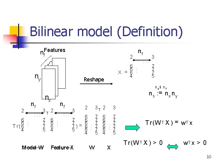
Bilinear model (Definition) nf. Features 2 ny 6. . 6 X = 6. 4 Reshape nf : : : 3 7 7 7 5 ns£ nf 2 6. . 6 T r (6. 4 nf : : : nx 3 T 2 7 7 7 5 Model W 6. 6 4 n s : = n x n y nf : : : 3 2 3 T 2 6 7 7 = 6. . 7 7) 6. 7 6 7 5 4 5 Feature X w 3 6 7 6. . 7 6 7 4 5 x T r (W T X ) = w. T x T r (W T X ) > 0 w. T x > 0 10

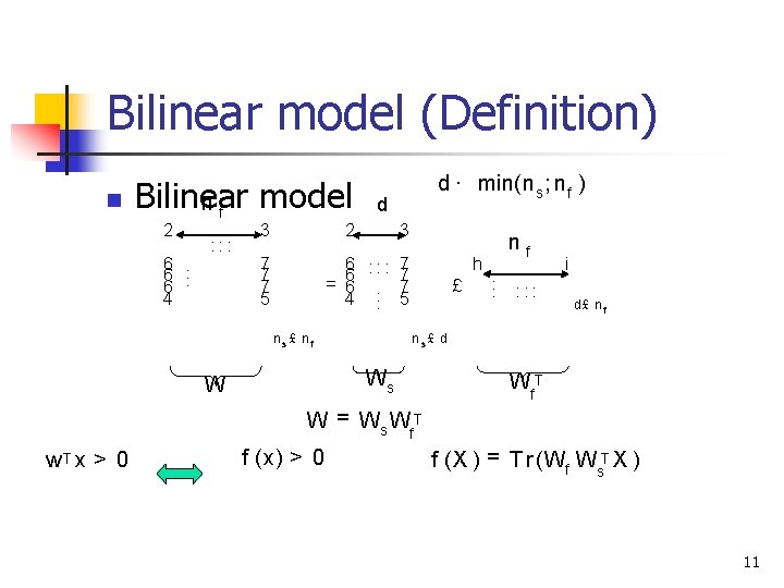
Bilinear model (Definition) n Bilinear model nf 2 6. 6 4 : : : 3 d 2 7 7 7 5 d · min(n s ; n f ) 3 6 : : : 7 7 = 6 6. . 7 4. 5 ns£ nf h £ . . . : : : i d£ n f ns£ d Ws W nf Wf. T W = Ws Wf. T w. T x > 0 f (x) > 0 f (X ) = T r (Wf Ws. T X ) 11

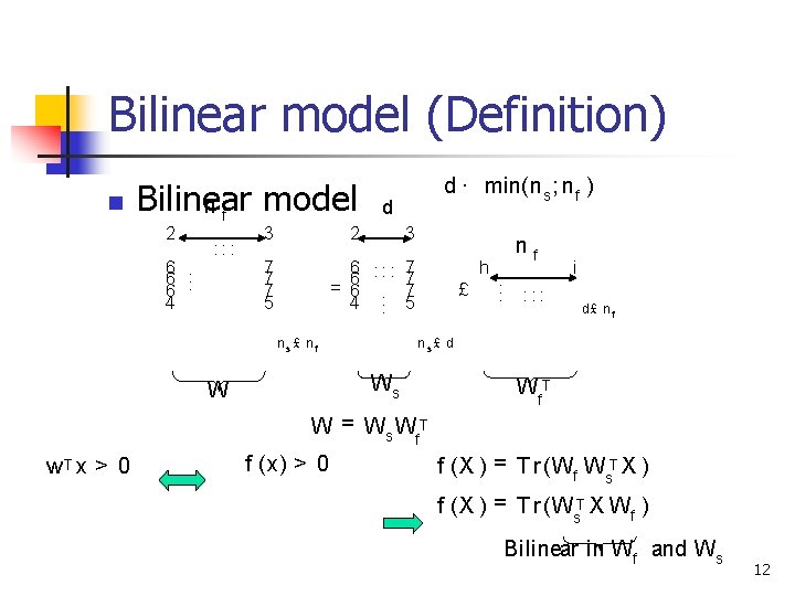
Bilinear model (Definition) n Bilinear model nf 2 6. 6 4 : : : 3 d 2 7 7 7 5 d · min(n s ; n f ) 3 6 : : : 7 7 = 6 6. . 7 4. 5 ns£ nf h £ . . . : : : i d£ n f ns£ d Ws W nf Wf. T W = Ws Wf. T w. T x > 0 f (x) > 0 f (X ) = T r (Wf Ws. T X ) f (X ) = T r (Ws. T X Wf ) Bilinear in Wf and Ws 12

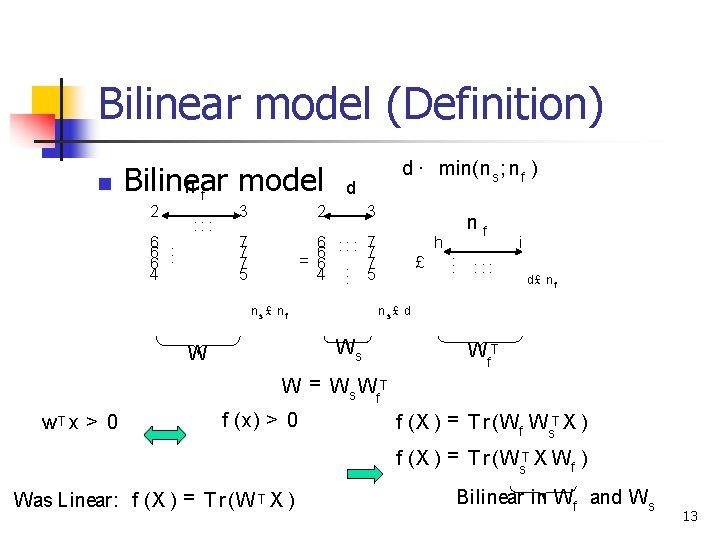
Bilinear model (Definition) n Bilinear model nf 2 6. 6 4 : : : 3 d 2 7 7 7 5 d · min(n s ; n f ) 3 6 : : : 7 7 = 6 6. . 7 4. 5 ns£ nf h £ . . . : : : i d£ n f ns£ d Ws W nf Wf. T W = Ws Wf. T w. T x > 0 f (x) > 0 f (X ) = T r (Wf Ws. T X ) f (X ) = T r (Ws. T X Wf ) Was Linear: f (X ) = T r (W T X ) Bilinear in Wf and Ws 13

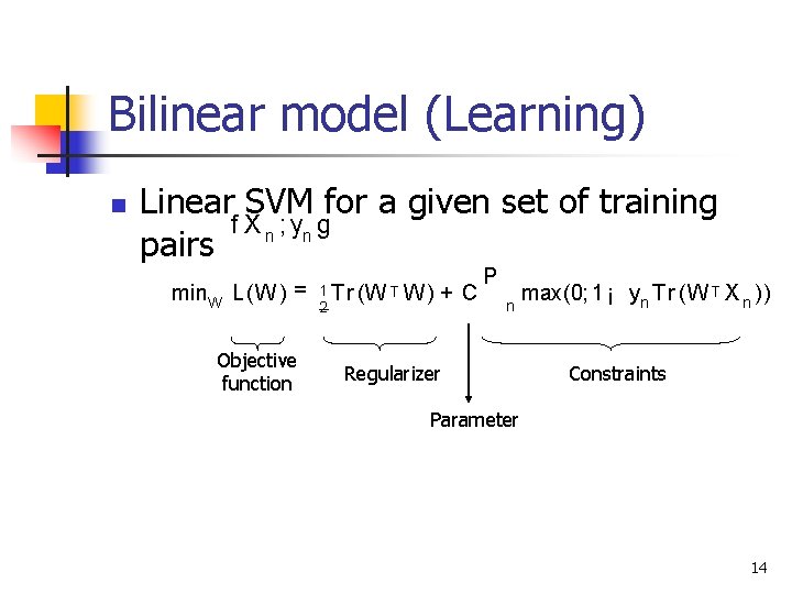
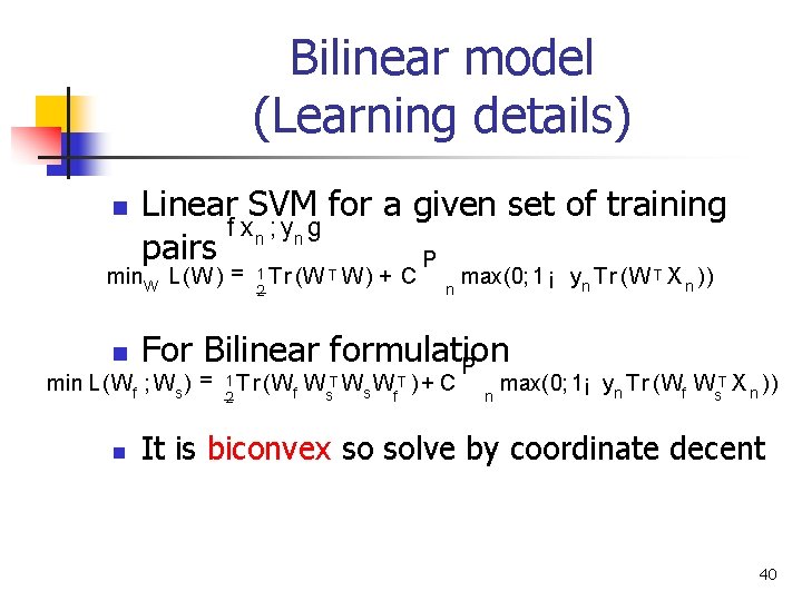
Bilinear model (Learning) n Linear SVM for a given set of training f X n ; yn g pairs min. W L (W ) = Objective function 1 T r (W T W ) 2 + C P n Regularizer max(0; 1 ¡ yn T r (W T X n )) Constraints Parameter 14

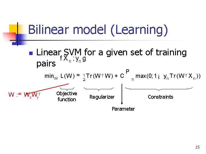
Bilinear model (Learning) n Linear SVM for a given set of training f X n ; yn g pairs min. W W : = Ws Wf. T L (W ) = Objective function 1 T r (W T W ) 2 + C P n Regularizer max(0; 1 ¡ yn T r (W T X n )) Constraints Parameter 15

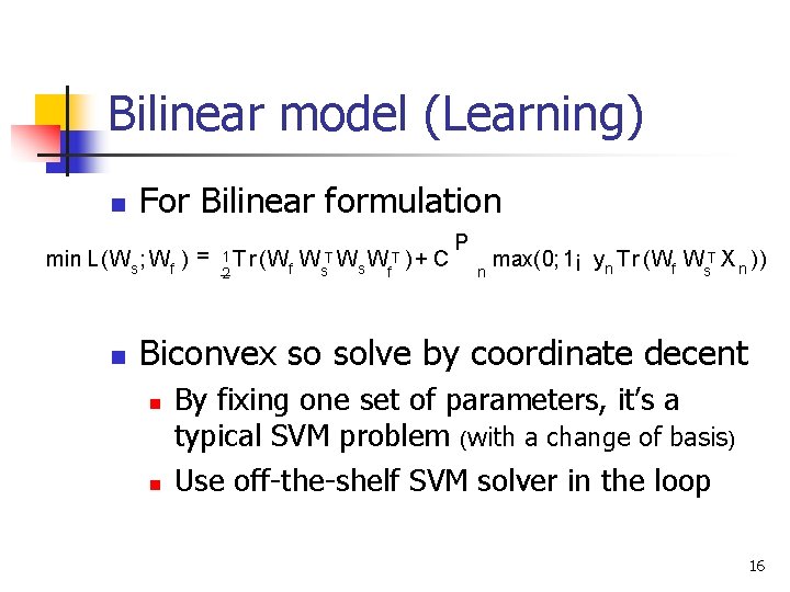
Bilinear model (Learning) n For Bilinear formulation min L (Ws ; Wf ) = n 1 T r (W f 2 Ws. T Ws Wf. T ) + C P n max(0; 1¡ yn T r (Wf Ws. T X n )) Biconvex so solve by coordinate decent n n By fixing one set of parameters, it’s a typical SVM problem (with a change of basis) Use off-the-shelf SVM solver in the loop 16

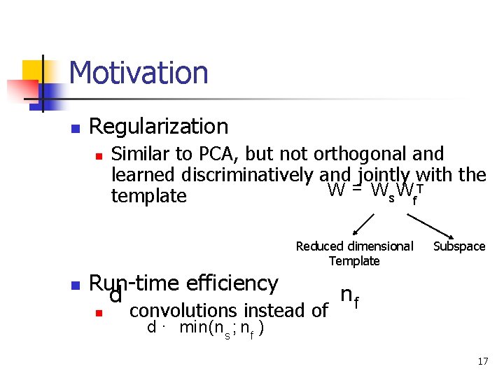
Motivation n Regularization n Similar to PCA, but not orthogonal and learned discriminatively and jointly with the W = Ws Wf. T template Reduced dimensional Template n Run-time efficiency n d convolutions instead of Subspace nf d · min(n s ; n f ) 17

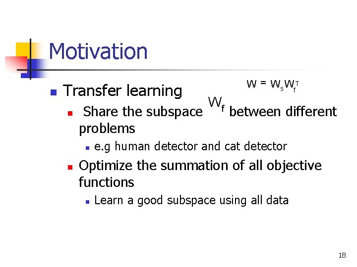
Motivation n Transfer learning n Share the subspace problems n n W = Ws Wf. T Wf between different e. g human detector and cat detector Optimize the summation of all objective functions n Learn a good subspace using all data 18

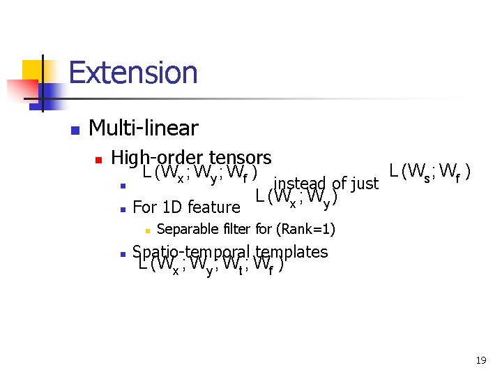
Extension n Multi-linear n High-order tensors n n L(Ws ; Wf ) L (Wx ; Wy ; Wf ) instead of just L (Wx ; Wy ) For 1 D feature n n Separable filter for (Rank=1) Spatio-temporal templates L(Wx ; Wy ; Wt ; Wf ) 19

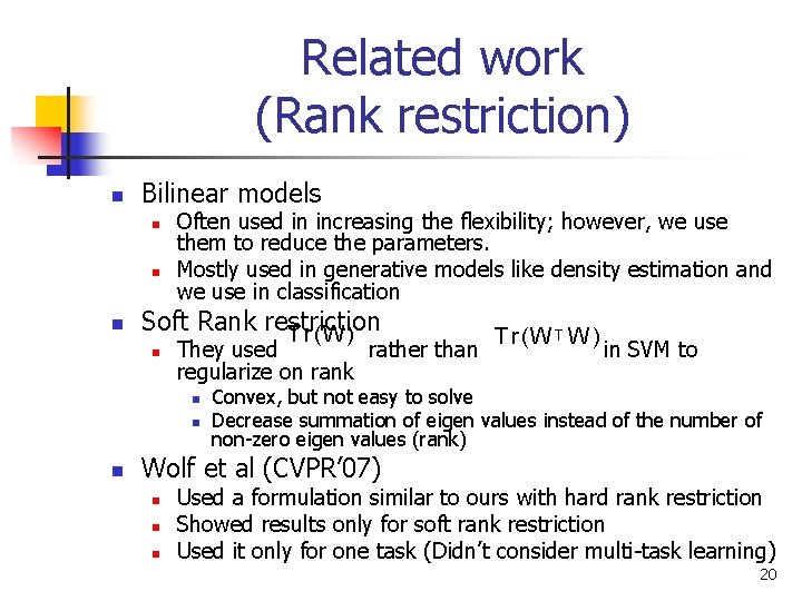
Related work (Rank restriction) n Bilinear models n n n Often used in increasing the flexibility; however, we use them to reduce the parameters. Mostly used in generative models like density estimation and we use in classification Soft Rank restriction T r (W ) n They used rather than regularize on rank n n n T r (W T W ) in SVM to Convex, but not easy to solve Decrease summation of eigen values instead of the number of non-zero eigen values (rank) Wolf et al (CVPR’ 07) n n n Used a formulation similar to ours with hard rank restriction Showed results only for soft rank restriction Used it only for one task (Didn’t consider multi-task learning) 20

Related work (Transfer learning) n Dates back to at least Caruana’s work (1997) n n n We got inspired by their work on multi-task learning Worked on: Back-propagation nets and k-nearest neighbor Ando and Zhang’s work (2005) n n n Linear model All models share a component in low-dimensional subspace (transfer) Use the same number of parameters 21

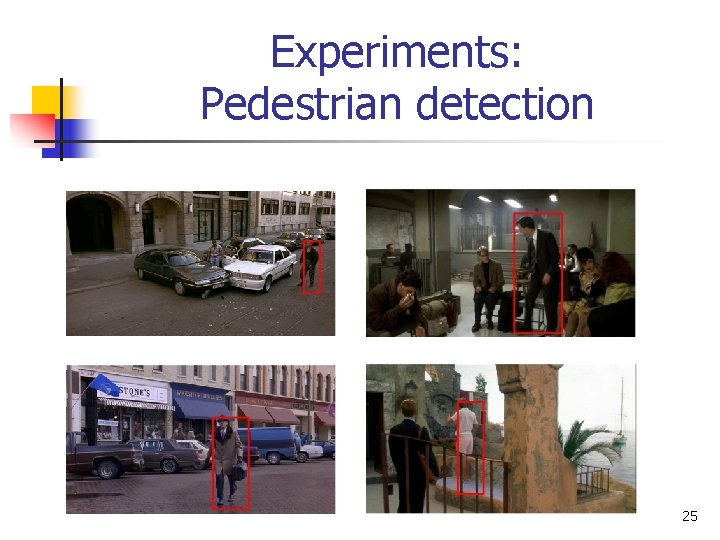
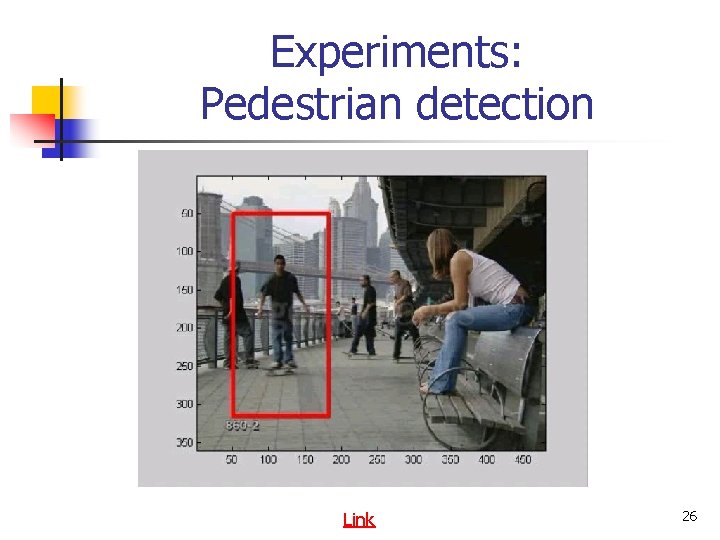
Experiments: Pedestrian detection n Baseline: Dalal and Triggs’ spatiotemporal classifier (ECCV’ 06) n Linear SVM on features: n n n (84 for each 8£ 8 cell) Histogram of gradient (HOG) Histogram of optical flow Made sure that the spatiotemporal is better than the static one by modifying the learning method 22

Experiments: Pedestrian detection n Dataset: INRIA motion and INRIA static n n n 3400 video frame pairs 3500 static images Typical values: = n s 14 £ 6, n f = 84, d = 5 or 10 n n Evaluation n Average precision Initialize with PCA in feature space Ours is 10 times faster 23

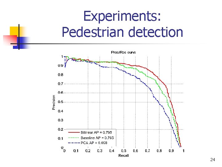
Experiments: Pedestrian detection 24

Experiments: Pedestrian detection 25

Experiments: Pedestrian detection Link 26

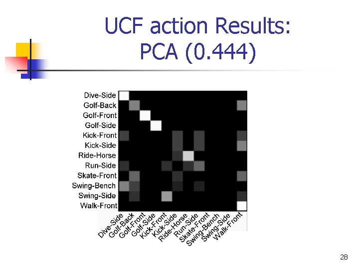
Experiments: Human action classification 1 n n 1 vs all action templates Voting: n n A second SVM on confidence values Dataset: n n n UCF Sports Action (CVPR 2008) They obtained 69. 2% We got 64. 8% but n n More classes: 12 classes rather than 9 Smaller dataset: 150 videos rather than 200 Harder evaluation protocol: 2 -fold vs. LOOCV 87 training examples rather than 199 in their case 27

UCF action Results: PCA (0. 444) 28

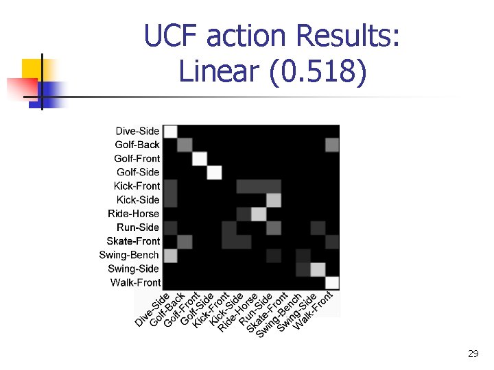
UCF action Results: Linear (0. 518) 29

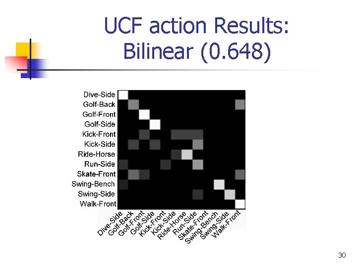
UCF action Results: Bilinear (0. 648) 30

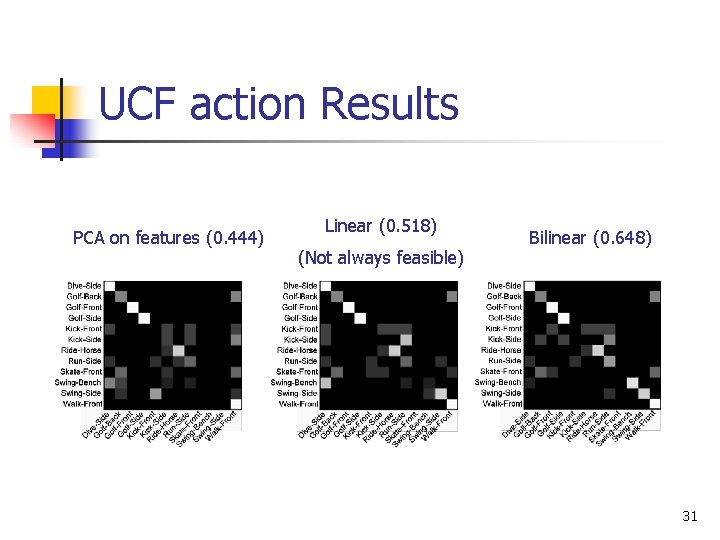
UCF action Results PCA on features (0. 444) Linear (0. 518) (Not always feasible) Bilinear (0. 648) 31

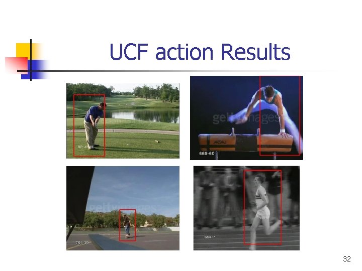
UCF action Results 32

Experiments: Human action classification 2 n Transfer n n n We used only two examples for each of 12 action classes Once trained independently Then trained jointly n n Shared the subspace Adjusted the C parameter for best result 33

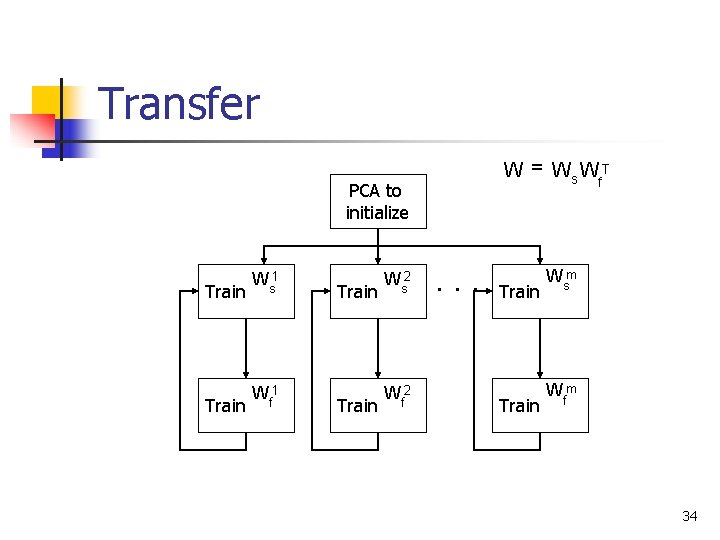
Transfer PCA to initialize Train Ws 1 Train Wf 1 Train Ws 2 Train Wf 2 W = Ws Wf. T Train Wsm Train Wfm 34

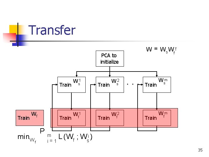
Transfer PCA to initialize Train Wf min. W P f m i= 1 Train Ws 1 Train Wf 1 Train Ws 2 Train Wf 2 W = Ws Wf. T Train Wsm Train Wfm L (Wf ; Wsi ) 35

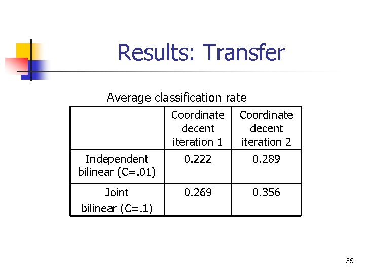
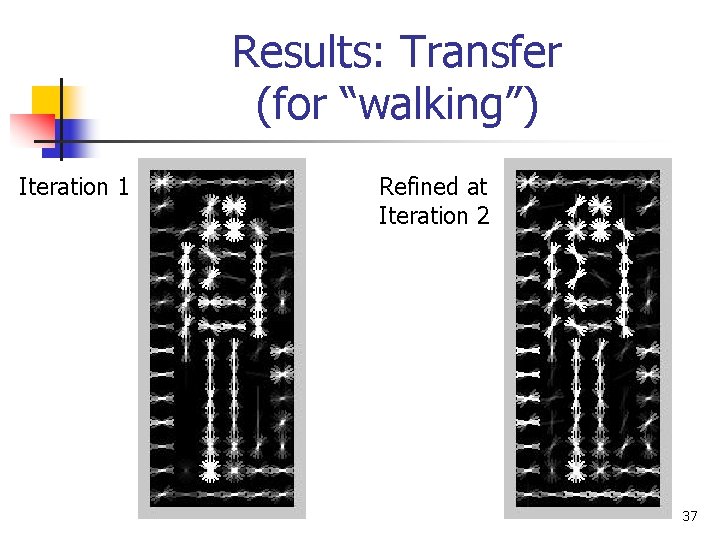
Results: Transfer Average classification rate Coordinate decent iteration 1 Coordinate decent iteration 2 Independent bilinear (C=. 01) 0. 222 0. 289 Joint bilinear (C=. 1) 0. 269 0. 356 36

Results: Transfer (for “walking”) Iteration 1 Refined at Iteration 2 37

Conclusion n Introduced multi-linear classifiers n n n Exploit natural matrix/tensor representation of spatiotemporal data Trained with existing efficient linear solvers Shared subspace for different problems n A novel form of transfer learning n Got better performance and about 10 X speed up in run-time compared to the linear classifier. Easy to apply to most high dimensional features n Simple: ~ 20 lines of Matlab code n (instead of dimensionality reduction methods like PCA) 38

Thanks! 39

Bilinear model (Learning details) n Linear SVM for a given set of training f x n ; yn g pairs P min. W L (W ) = 1 T r (W T W ) 2 + C n max(0; 1 ¡ yn T r (W T X n )) For Bilinear formulation P n min L (Wf ; Ws ) = n 1 T r (W f 2 Ws. T Ws Wf. T ) + C n max(0; 1¡ yn T r (Wf Ws. T X n )) It is biconvex so solve by coordinate decent 40

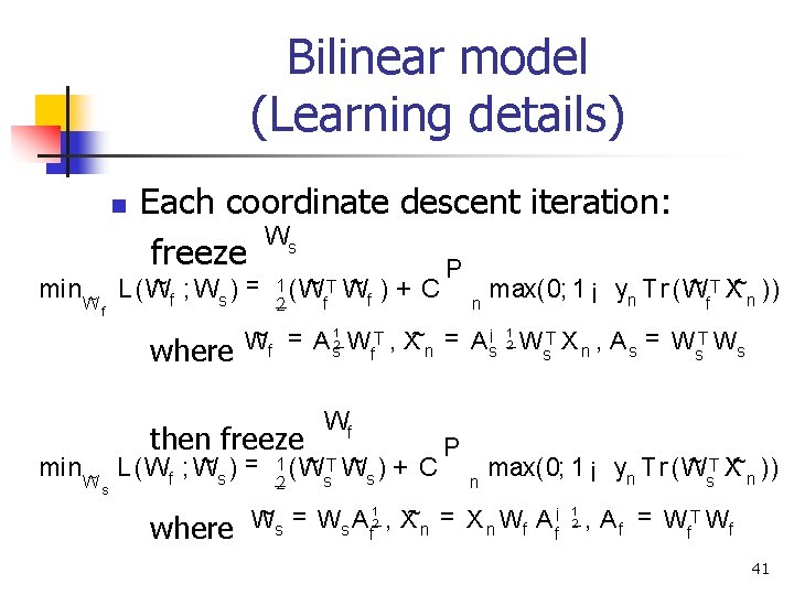
Bilinear model (Learning details) n Each coordinate descent iteration: Ws freeze P ~ ; W ) = min ~ L ( W f s Wf where min ~ Ws ~TW ~ 1 (W f f 2 n ~ T X~ )) max(0; 1 ¡ yn T r ( W n f ~ = A 12 W T , X~ = A ¡ 12 W T X , A = W T W W s s n n s s f then freeze ~ )= L (Wf ; W s where )+ C Wf ~T 1 (W s 2 ~ )+ C W s P n ~ T X~ )) max(0; 1 ¡ yn T r ( W n s ~ = W A 12 , X~ = X W A ¡ W s s f n n f f 1 2 , A f = Wf. T Wf 41