BIJU P M PGT ECONOMICS KV 2 KOCHI

BIJU P M PGT ECONOMICS KV 2, KOCHI

Production The theory of the firm describes how a firm makes costminimizing production decisions and how the firm’s resulting cost varies with its output. The Production Decisions of a Firm The production decisions of firms are analogous to the purchasing decisions of consumers, and can likewise be understood in three steps: 1. Production Technology 2. Cost Constraints 3. Input Choices The aim of the producer is to get maximum profit. 3

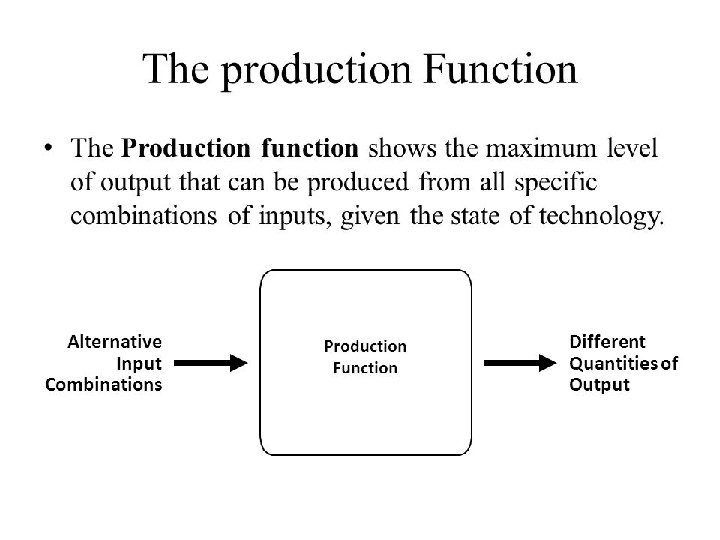
THE TECHNOLOGY OF PRODUCTION ● Factors of production - Inputs into the production process (e. g. , labor, capital, and materials) The Production Function Means The technological relationship between inputs(Land, Labour, Capital and Organization) and outputs. ● Production function - Function showing the highest output that a firm can produce for every specified combination of inputs Inputs and outputs are flows. Production functions describe what is technically feasible when the firm operates efficiently. ISOQUANT: Alternative way of representing the Production Function is called Isoquant. It is the set of possible combinations of two Inputs that yield the same possible level of ouput. 4

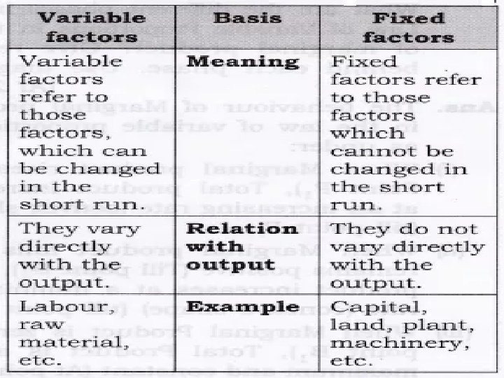
THE TECHNOLOGY OF PRODUCTION The Short Run versus the Long Run ● Short run - Period of time in which quantities of one or more production factors cannot be changed ● Fixed input - Production factor that cannot be varied ● Long run - Amount of time needed to make all production inputs variable 5
 returns A more units of the variable factor are")
The law of diminishing (marginal) returns A more units of the variable factor are used, there will come a point where additional units of the variable factor will produce less than previous units. 9

Wheat production per year from a particular farm Tonnes of wheat produced per year d TPP Maximum output Diminishing returns set in here b Number of farm workers 10
 = TPP/ L TPn –TPn-1 OR MP is")
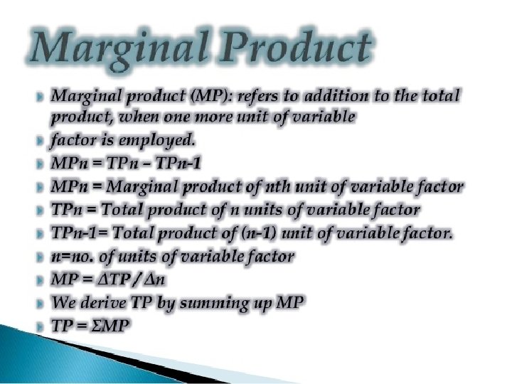
Short-run production Marginal physical product (MPP) = TPP/ L TPn –TPn-1 OR MP is additional output attributed to an additional unit of the variable factor, other factors remaining constant. 11

Tonnes of wheat per year Wheat production per year from a particular farm TPP = 7 Number of farm workers (L) L = 1 Number of farm workers (L) 12
 Tonnes of wheat per year Wheat production per")
TPP Number of farm workers (L) Tonnes of wheat per year Wheat production per year from a particular farm Number of farm workers (L) MPP 13
 = TPP/L AP is output per unit of")
Short-run production Average physical product (APP) = TPP/L AP is output per unit of the variable factor used in the process of production 14

15 Tonnes of wheat per year Shows Law of Variable Proportion Tonnes of wheat per year Wheat production per year from a particular farm TPP Number of farm workers (L) APP = TPP / L APP Number of farm workers (L) MPP

Tonnes of wheat per year Wheat production per year from a particular farm 16 TPP b Diminishing returns set in here Number of farm workers (L) b APP Number of farm workers (L) MPP

Tonnes of wheat per year Wheat production per year from a particular farm 17 d TPP b Maximum output Number of farm workers (L) b APP d Number of farm workers (L) MPP

Tonnes of wheat per year Wheat production per year from a particular farm 18 Slope = TPP / L = APP d c TPP b Number of farm workers (L) b c APP d Number of farm workers (L) MPP
 Returns to factor OR Law of variable proportion")
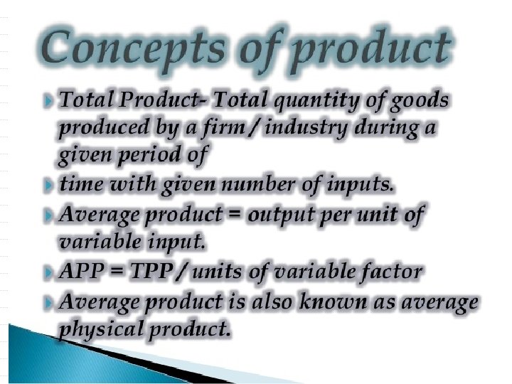
PRODUCTION WITH ONE VARIABLE INPUT (LABOR) Returns to factor OR Law of variable proportion Average and Marginal Products ● Average product - Output per unit of a particular input ● Marginal product - Additional output produced as an input is increased by one unit Average product of labor = Output/labor input = q/L Marginal product of labor = Change in output/change in labor input = Δq/ΔL 19

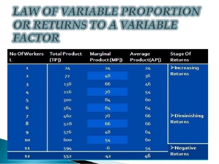
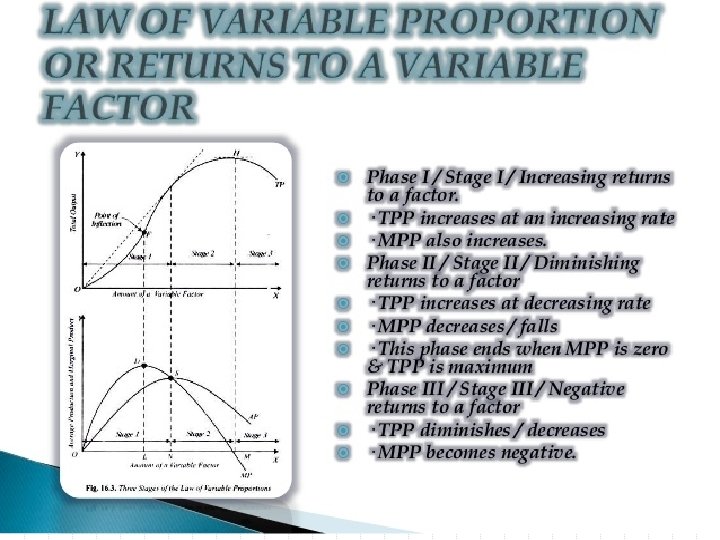
Returns to factor OR Law of variable proportion Three stages of production: Stage I: - In this stage TP increase at an increasing rate, MP and AP also increase. Therefore this stage is an increasing stage. Stage II: - In the IInd stage TP increases at a deceasing rate, MP falls but positive AP also starts to fall. Therefore know as decreasing stage. The point at which TP start to increase at decreasing rate is known as point of inflexion. Stage III: -TP, AP and MP fall in this stage. MP becomes negative and therefore this stage is known as negative stage. The law can be explained with the help of following table and diagram. 20
 TABLE. Production with One Variable Input Amount of")
PRODUCTION WITH ONE VARIABLE INPUT (LABOR) TABLE. Production with One Variable Input Amount of Labor (L) of Capital (K) Total Average Output (q) Product (q/L) Marginal Product (∆q/∆L) 0 10 0 — — 1 10 10 2 10 30 15 20 3 10 60 20 30 4 10 80 20 20 5 10 95 19 15 6 10 108 18 13 7 10 112 16 4 8 10 112 14 0 9 10 108 12 4 10 10 10 8 21
 The Slopes of the Product Curve Production with")
PRODUCTION WITH ONE VARIABLE INPUT (LABOR) The Slopes of the Product Curve Production with One Variable Input The total product curve in (a) shows the output produced for different amounts of labor input. The average and marginal products in (b) can be obtained (using the data in Table 6. 1) from the total product curve. At point A in (a), the marginal product is 20 because the tangent to the total product curve has a slope of 20. At point B in (a) the average product of labor is 20, which is the slope of the line from the origin to B. The average product of labor at point C in (a) is given by the slope of the line 0 C. 22
 The Slopes of the Product Curve Production with")
PRODUCTION WITH ONE VARIABLE INPUT (LABOR) The Slopes of the Product Curve Production with One Variable Input (continued) To the left of point E in (b), the marginal product is above the average product and the average is increasing; to the right of E, the marginal product is below the average product and the average is decreasing. As a result, E represents the point at which the average and marginal products are equal, when the average product reaches its maximum. At D, when total output is maximized, the slope of the tangent to the total product curve is 0, as is the marginal product. 23
 The Law of Diminishing Marginal Returns ● law")
PRODUCTION WITH ONE VARIABLE INPUT (LABOR) The Law of Diminishing Marginal Returns ● law of diminishing marginal returns Principle that as the use of an input increases with other inputs fixed, the resulting additions to output will eventually decrease. The Effect of Technological Improvement Labor productivity (output per unit of labor) can increase if there are improvements in technology, even though any given production process exhibits diminishing returns to labor. As we move from point A on curve O 1 to B on curve O 2 to C on curve O 3 over time, labor productivity increases. 24

After the addition to a variable factor we find the following Three Situations : 1. Increase in product at increasing rates : (Increasing returns to variable factors) 2. Increase in product at constant rate (Constant return to variable factor) 3. Increase in product at decreasing rate (Diminishing or decreasing return to variable factor) 25

OR LAWS OF VARIABLE PROPORTIONS It shows the relationship between input and output in short period in which only one factor is changed keeping other inputs fixed as a result the ratio between fixed and variable factor changes. The law states that as the proportion of factors is changed TP at first increases more than proportionately, then proportionately and finally less than proportionately. When more and more units of variable factors are applied along with fixed factor, the production passes through three stages. 26 Law of Variable Proportions- The law states that if we go on using more and more units of a variable factor (Labour) with a fixed factor( land , Capital) the total output initially increases at an increasing rate but beyond certain point, it increases at a diminishing rate and finally it falls.

I Stage: Initially TP increases at increasing rate, AP and MP both increases. II Stage : TP increases at diminishing rate MP starts falling up to zero but remain positive, AP also fall. AP = MP then AP is maximum. III Stage: TP fall, MP become negative, AP also falls but remains positive. 27

LAWS OF RETURNS: It shows the relationship between inputs and output in short period where one variable is changed keeping other factors constant. These are all Three Laws of Returns. 1)Laws of increasing returns to a factor: It occurs when TP increases at increasing rate marginal product increase due to increase in variable factor. 2) Law of constant returns to a factor: It occurs when additional application of the variable factors increases. 3)Law of diminishing returns to a factor: It is a situation in which TP increases at decreasing rate and MP decreases. When more units of variable factors are combined with the fixed factor. 28

LAW OF RETURNS It shows the relationship between inputs and output in short period where on variable is changed keeping other factor constant. These are three laws of returns 29

30

CAUSES OF INCREASING RETURNS TO A FACTOR Fuller utilization of fixed factor Increased efficiency of the variable factor due to better division of labor. Better coordinators between the factor. Y MP Labour TP MP 40 1 20 20 30 2 45 25 3 75 30 4 115 40 5 165 50 20 10 0 ------- MP 50 1 2 3 Unit of labour 4 5 X 31

Causes of constant returns to a factor Operation of law of diminishing returns Optimum use of fixed factor Lack of perfect substitution between the factors Product Y Labour TP MP AP 1 25 25 25 2 50 25 25 20 3 75 25 25 10 4 100 25 25 5 125 25 25 MP=AP 30 0 1 2 3 Unit of labour X 32

Causes of diminishing returns to a factor Beyond the optimum utilization of fixed factors. Imperfect factors substitutability. Poor coordination between the fixed and variable factors. Y 1 2 ---- o MP ------------- 10 ------40 -------30 -------------20 50 3 4 Unit of labour Land TP MP 5 X MP 1 5 50 50 2 5 90 40 3 5 120 30 4 5 145 25 5 5 165 20 33

Assumption One of the factor is variable are fixed while other factors are variable Units of variable factors are increased one by one and all units are homogenous There is no change in the technique of production. Factors of production can be used in fact different proportion. 34

BIJU P MPGT ECONOMICS KV 2 , KOCHI
- Slides: 42