BIJU P M PGT ECONOMICS KV 2 KOCHI

BIJU P M PGT ECONOMICS KV 2, KOCHI

Introduction To Consumer equilibrium A consumer is one who buys goods and services For satisfaction of wants. The objective of a consumer is to get maximum satisfaction from spending his income on various goods and services given prices. Due to limited resources , consumer is not able to satisfy all his needs. He will try to get maximum satisfaction by spending his income on various goods and services Two approaches are used for getting an answer to this question. (1) Utility approach (2) Indifference approach

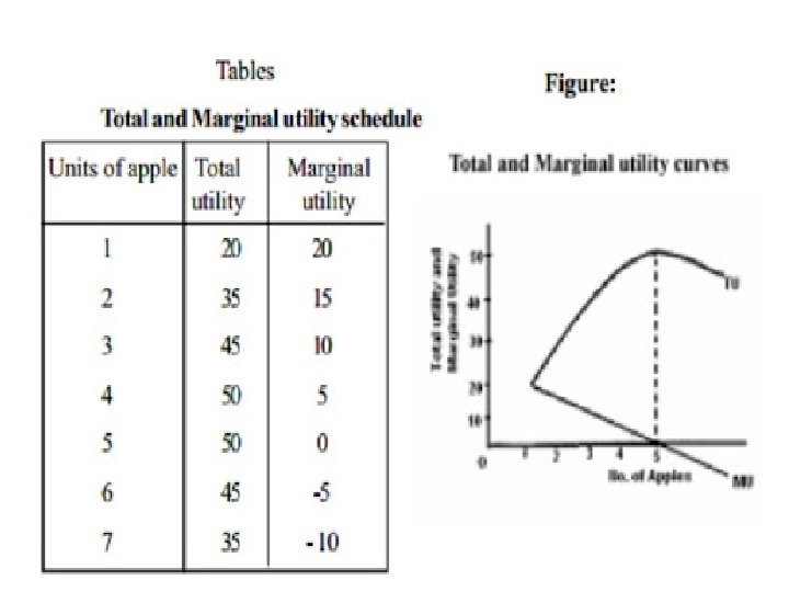
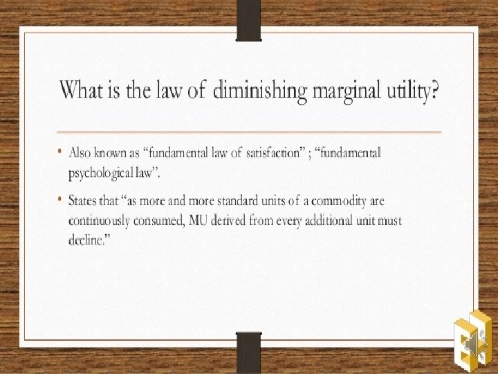
What is Utility : The term ‘Utility’ refers to the want satisfying power of a commodity. It means expected satisfaction to a consumer when he is willing to spend money on a stock of commodity which has the capacity to satisfy his want. Total Utility: - The total psychological satisfaction obtained by a consumer gets from a given commodity/service. (or) Sum of marginal utility is known as total utility. (TU = £MUs) Marginal Utility: - An addition made to total utility by consuming an extra unit of commodity. Sum of marginal utilities various goods is known as total utility. MU =ΔTU Law of Diminishing Marginal Utility: - It states that as the consumer consume more and more units of a commodity , the marginal utility gets from each successive units goes on diminishing

 TUx 1 100")
Marginal Utility Estimation of MU schedule from TU schedule Unit (X) TUx 1 100 2 MU =ΔTU Solution : Unit (X) TUx MUx 190 1 100 3 260 2 190 90 4 310 3 260 70 5 350 4 310 50 5 350 40

Law of Diminishing Marginal Utility 20 162 6 16 178 7 6 184 8 4 188 9 0 188 10 -10 178 ______-_______ 5 TU/MU The relationship between total utility , MU, and the law of diminishing MU can be presented through the following table. Y TU increases Unit MU TU as long as MU 200 consumed £MU Diagram is positive. (Bread) 188 _ _ _____ _ _ 184 0 0 178 1 40 40 TU 162 2 38 78 142 3 36 114 4 28 142 80 40 20 0 1 2 3 4 5 6 7 8 9 10 Unit of Bread X MU


Consumer Equilibrium in case of One Commodity With the help of utility schedule: Consumer equilibrium refers to a situation when he spends his given income on purchase of a commodity ( or commodities) in such a way that yields him maximum satisfaction Condition of equilibrium: MU of product / Price of product = MU of a Rupee. consumer consumes different unit and obtain satisfaction in following manner : MU (-) Price 56 48 No. of units consumed MU Price Extra Utility(Profit) 1 40 16 24 2 38 16 22 3 36 16 20 4 28 16 12 5 20 16 4 6 16 16 0 7 6 16 - 10 Consumer Equilibrium 40 32 24 E 16 Price ______ Schedule 8 1 2 3 4 5 6 MU 7

Assumptions for Consumer equilibrium Consumer behaviour is rational Consumer behaviour is consistent i. e. it does not change frequently : There are two commodities in consideration for determination of consumer equilibrium

Marginal Utility of money Marginal utility of money refers to ‘worth of rupee’ to a consumer. Example : If A rupee can buy 100 gms of sugar, 500 gms of rice , and 500 gms of salt (which represent a standard basket of goods to the consumer) and if total utility from these goods is (say) 50 utils, then 50 is to be taken as marginal utility of money.
Introduction The Indifference Curve Analysis is an alternative explanation of the")
Indifference Curve Analysis (A)Introduction The Indifference Curve Analysis is an alternative explanation of the consumer’s behaviour. It is an alternative in two respects : Different assumptions and different tools. Let us see how assumptions and tools are different.

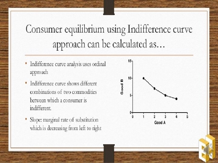
The Utility analysis is assumed as cardinal i. e. the utility is expressed in exact units as 1, 2, 3 etc. The Indifference Curve analysis is assumed as Ordinal as the Utility is expressed as first , second , third , etc. The assumption of Ordinal Utility is more realistic than the assumption of cardinal utility. In this respect, the Indifference curve analysis is considered to be an Improvement over the Utility Analysis.


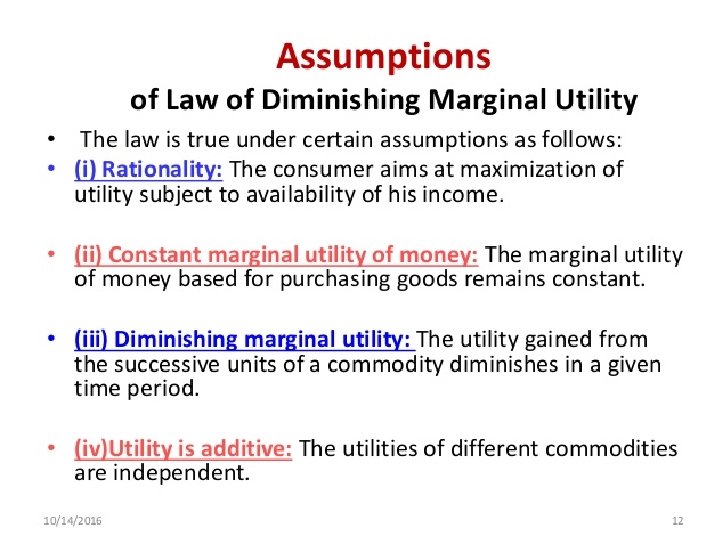
Consumers equilibrium • The main objective of the consumers to get maximum satisfaction. • A consumer is in equilibrium where he gets maximum satisfaction out of his income, and he has no tendency to change in his pattern of consumption. • Consumers equilibrium by utility analysis is based upon the following assumptions: Consumer is rational. Utility can be measured cardinally. Marginal utility of money remains constant. Income of the consumer and price of the commodity remain fixed No change in the taste and preferences of the consumer. Consumer has the perfect knowledge.

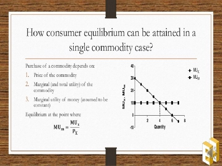
Determination of Consumers equilibrium. I. Under single commodity: When a consumer purchase a commodity he will be in equilibrium position at a point where marginal utility of the commodity is equal to its price, the following condition is fulfilled: Marginal utility = price Purchase of the commodity by a consumer depends on 3 factors: ü Price of the commodity. ü Marginal utility of Money is the extra utility derived when an additional rupee is spend on available goods. Let the MUM is 1 util Consumer consume commodity X Let the price PX is 6
 MU (utils) 1 10 2")
Determination of Consumers equilibrium. Marginal utility schedule X (units) MU (utils) 1 10 2 8 3 7 4 6 5 3 6 0 When consumer consume 1 unit of commodity MUM is 1 util MUMx is 10 (worth of Rs. 10) Px is 6 Consumer pays Rs 6 but he gets consumption Worth of 10 utils, When consumer consume 2 units of the commodity Worth of a rupee is 1 util MUx is 8 that is worth of Rs. 8 But he pays Rs 6 when he pays less and get utility More he continuous consumption. When consumer consume 4 units of the commodity Worth of a rupee is 1 util MUx is 6 that is worth of Rs. 6 Here MUx = Px

• The consumer will be in equilibrium when he consumes 4 units of the commodity where, The general principle of consumer’s equilibrium: OR

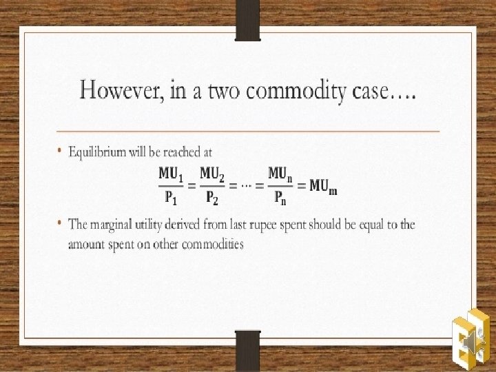
Consumers equilibrium- under two commodities • • Suppose a consumer consumes only two goods. Let these goods be X and Y Prices Px and Py. Consumer attains equilibrium only when the following condition is satisfied: MUx Px = MUy = M. U m or M U of a rupee spent on a good Py MUx = Marginal utility of good X MUy = Marginal utility of a good Y Px = Price of good X Py = Price of good Y M U. m =. Marginal utility of money The assumption of consumer’s equilibrium for one good is extended to two good also.

CONSUMER’S EQUILIBRIUM TWO GOODS… • What happens when Suppose a consumer has Rs. 30 with him which he wants to spend on two goods X and Y. The price of each unit of good is Rs. 4 and Rs. 2 Units MUx MU/Px MUy Muy/py 1 80 80/4=20 40 40/2=20 2 72 18 38 19 3 64 16 36 18 4 56 14 34 17 5 48 12 32 16 6 40 10 30 15 7 32 8 28 14 8 24 6 26 12

Consumers equilibrium • Consumer will be in equilibrium when he purchase 4 units of good X and 7 units of good Y. This can be stated in the following ways: • From the table (1) Thus the condition (2) (3) and is satisfied

CONSUMER’S EQUILIBRIUMFOR MORE THAN TWO GOODS • Equilibrium condition for more than two goods:

An Indifference Schedule is a table showing different combinations of the goods such that utility from each combination is the same. Assumptions (i) As the quantity of one good is increased , quantity of the other good must be decreased. (ii) As the Quantity of one good goes on increasing, the quantity of the other good not only decreases, but decreases at a decreasing rate.

Combination Soft Drinks Chocolate A 4 14 B 5 10 C 6 08 D 8 06 E 12 05
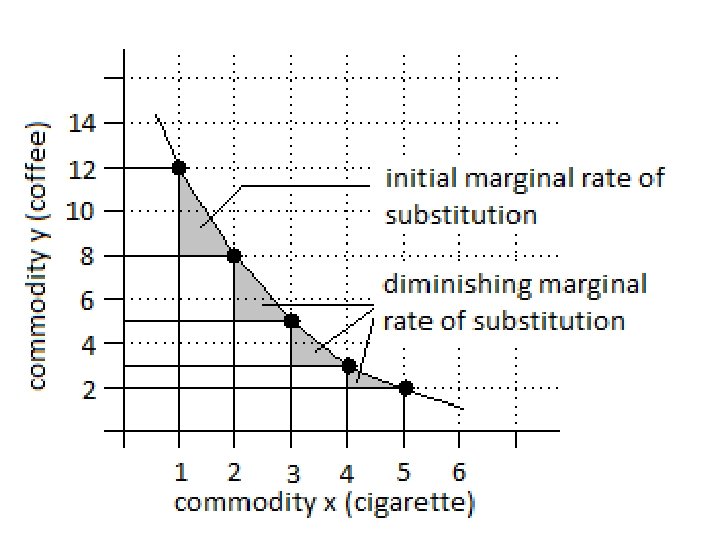

MRS is a rate at which the consumer is willing to sacrifice on good to Obtain one more unit of the other good. Combination A MRS - B C 1 X : 4 Y 1 X : 2 Y D E 2 X : 2 Y 4 X : 1 Y With reference to the Table 1. MRS = Change in the q. ty of good sacrificed. Change in the q. ty of good obtained. For Example , for the combination B MRS = Y X => - 4/1 = 4 (absolute value)

Moving along an IC we find that one good is substituted for others. The rate at which One more unit of Good-1 (on the X –axis) is substituted for Good-2 (on the Y-axis) is called MRS. R ∆Good-2 * A C* *B ∆Good -1 S O M IC N GOOD -1 MRS is always diminishing. ∆Good -1 loses GOOD-2 We take two points A&B on the adjoining IC. At point A, a consumer gets combination Of OR(=MA) of good 2, & OM(=RA) of good-2. Suppose he shifts to point B where he gets combination of OS(=MC) of good-2 and ON (=SB) of good-1. By this change he loses- AC(=MA-MC) amount of good-2 and (Gains=CB(ONOM)of good-1. which means he is willing to substitutegood-1 for good-2 at the rate of AC/CB. MRSxy = Y ∆Good-2 X
 Indifference Curve The Indifference curve is the locus of different combinations of")
(B 3) Indifference Curve The Indifference curve is the locus of different combinations of the two goods, the consumer consumes with each of the Combination having the same utility. Y Soft drinks Marginal rate of substitution of soft drinks for chocolate. X Soft Drinks

The set of all possible Indifference curves , the consumer has, is called Indifference map. The Indifference map is based on the assumption that the preferences are monotonic. Monotonic preferences mean that as consumption increases, total utility also increases along with it. Soft Drinks
 Sloping downwards from left to right. Because , to obtain more quantity of")
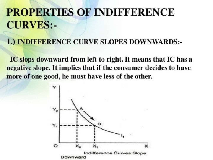
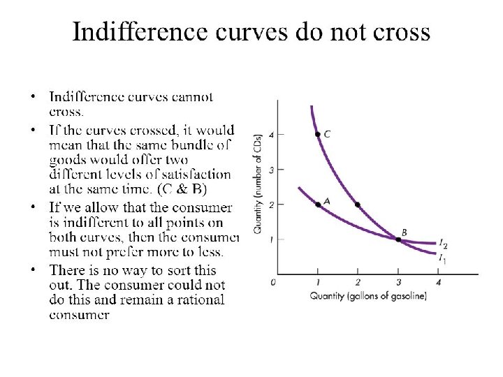
(i) Sloping downwards from left to right. Because , to obtain more quantity of one good , the consumer must give up some quantity of the other good in order to remain at the same utility level. (ii) Strictly convex towards the origin. Because , the MRS continuously declines as the consumer moves downwards along the curve. (iii) Higher Indifference curve represents higher utility. Because , assumptions are based on monotonic preferences. (IV) Two curves do not intersect to each other : If the intersect , the we get contradictory results in terms of preference ranking.

Budget set refers to the set of possible combinations of the two goods , the consumer consumes which he can afford from his income and given prices. This situation can be expressed in the form of an equation in the following way : Px. X + Py. Y < m The Equation is often referred to as Budget Constraint.
 The concept of Marginal Utility. (ii) The law of")
The Utility analysis uses (i) The concept of Marginal Utility. (ii) The law of diminishing marginal Utility. (iii) The law of Equi-marginal Utility. The Indifference curve analysis uses (i) The concept of Indifference Curve. (ii) Budget line.

A budget line is the Graphical presentation of the whole collection of the combinations of two goods , which costs the consumer exactly his income. Budget line is the locus of different combinations of two goods, which the consumer consumes and which cost the consumer exactly his income. The rate at which , the market requires sacrifices of one good to obtain extra unit of the other good is called Market Rate of Exchange (MRE).

Consumption Possibility Schedule Combinations Good X Good Y A 0 20 M. R. E 5 Y: 1 X B 1 15 5 Y: 1 X C 2 10 5 Y: 1 X D 3 05 5 Y: 1 X E 4 00 5 Y: 1 X

Graphical presentation MRE = Quantity of the good needed to be sacrificed Quantity of the good needed to be obtained Slope = Qty of the good sacrificed Qty of the good obtained Budget set Or Price of the good Obtained Price of the good Sacrificed = 3 Y = Px/Py X
 Change in the Income. (i)")
Budget line shifts because of the following changes. (a) Change in the Income. (i) If income Increases (ii) If Income Decreases A 1 A A A 2 B B 1 B 2 B
 Change in price of good X. (i) If price of Good X falls.")
(b) Change in price of good X. (i) If price of Good X falls. (ii) If price of Good X rises. A A B B 1 B 2 B
 Change in the price of Good Y. (ii) If the price of Good")
(c) Change in the price of Good Y. (ii) If the price of Good Y rises (i) If the price of Good Y falls. A 1 A A A 2 B B

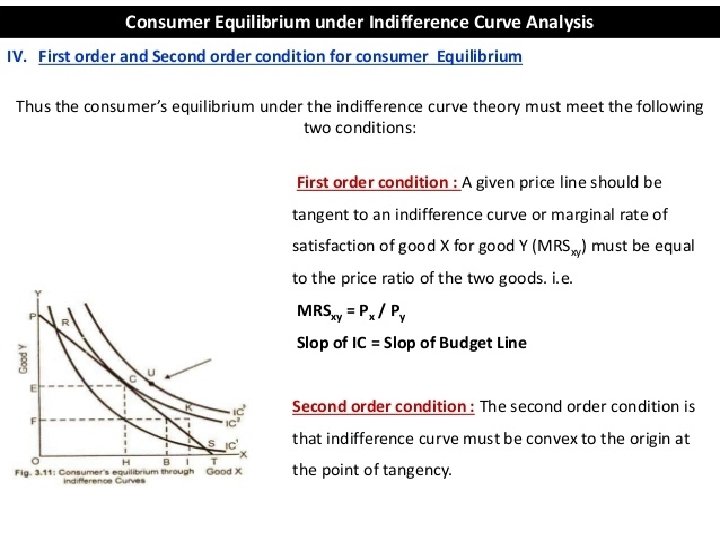
Consumer Equilibrium means the combination of Two goods , which the consumer can afford and which gives maximum satisfaction he possibly can get. A Consumer will be in equilibrium when the Indifference curve is tangent to the Budget line. The Consumer equilibrium will be at a point where the budget line meets the Indifference curve.
 The Consumer is rational. (b) The Utility is expressed ordinally. (c) MRS decreases")
(a) The Consumer is rational. (b) The Utility is expressed ordinally. (c) MRS decreases as more of one good is consumed by willingly sacrificing the other good. (d) Utility is increasing function of Consumption. (a)The Marginal Rate of Substitution (MRS) equals the Market Rate of Exchange (MRE). (b) MRS falls as more of one good is consumed in place of the other.

Graphical Presentation. Y Good Y A F y 1 G x 1 B X Good X

BIJU P MPGT ECONOMICS KV 2, KOCHI
- Slides: 54