Beyond Streams and Graphs Dynamic Tensor Analysis Jimeng
Beyond Streams and Graphs: Dynamic Tensor Analysis Jimeng Sun Dacheng Tao Speaker: Jimeng Sun Christos Faloutsos

Motivation Goal: incremental pattern discovery on streaming applications Streams: § E 1: Environmental sensor networks E 2: Cluster/data center monitoring § E 3: Social network analysis § Graphs: Tensors: § § § E 4: Network forensics E 5: Financial auditing E 6: f. MRI: Brain image analysis How to summarize streaming data effectively and incrementally?
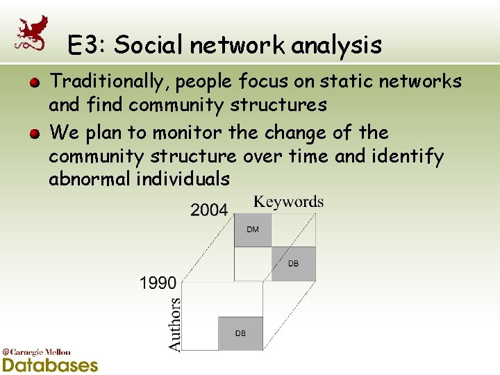
E 3: Social network analysis Traditionally, people focus on static networks and find community structures We plan to monitor the change of the community structure over time and identify abnormal individuals
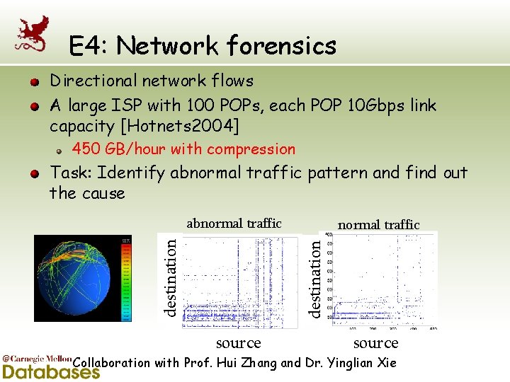
E 4: Network forensics Directional network flows A large ISP with 100 POPs, each POP 10 Gbps link capacity [Hotnets 2004] 450 GB/hour with compression Task: Identify abnormal traffic pattern and find out the cause normal traffic destination abnormal traffic source Collaboration with Prof. Hui Zhang and Dr. Yinglian Xie
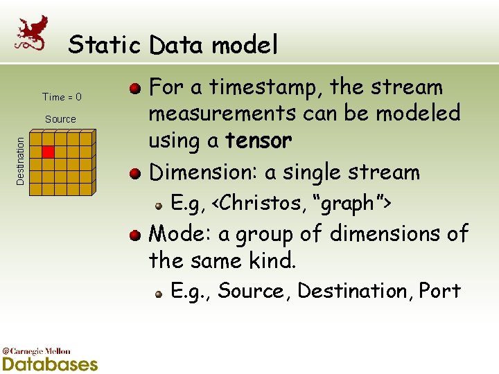
Static Data model Time = 0 Destination Source For a timestamp, the stream measurements can be modeled using a tensor Dimension: a single stream E. g, <Christos, “graph”> Mode: a group of dimensions of the same kind. E. g. , Source, Destination, Port
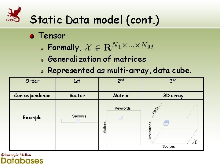
Static Data model (cont. ) Tensor Formally, Generalization of matrices Represented as multi-array, data cube. Order 1 st 2 nd 3 rd Correspondence Vector Matrix 3 D array Example
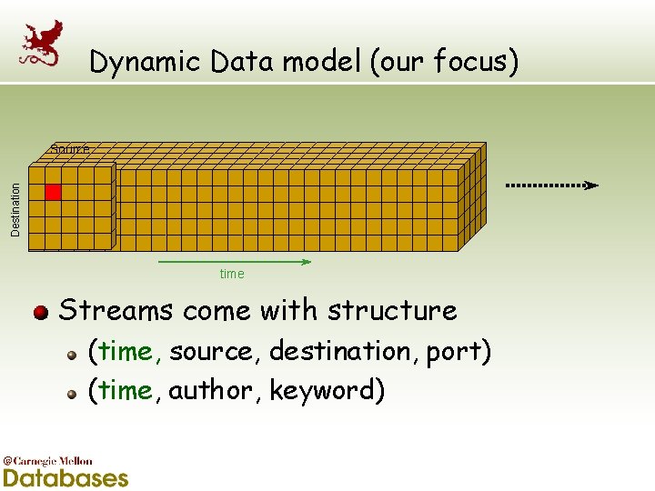
Dynamic Data model (our focus) Destination Source time Streams come with structure (time, source, destination, port) (time, author, keyword)

Dynamic Data model (cont. ) Tensor Streams A sequence of Mth order tensor where n is increasing over time Order 1 st 2 nd 3 rd Correspondence Multiple streams Time evolving graphs 3 D arrays e author time Example keyword tim … … …
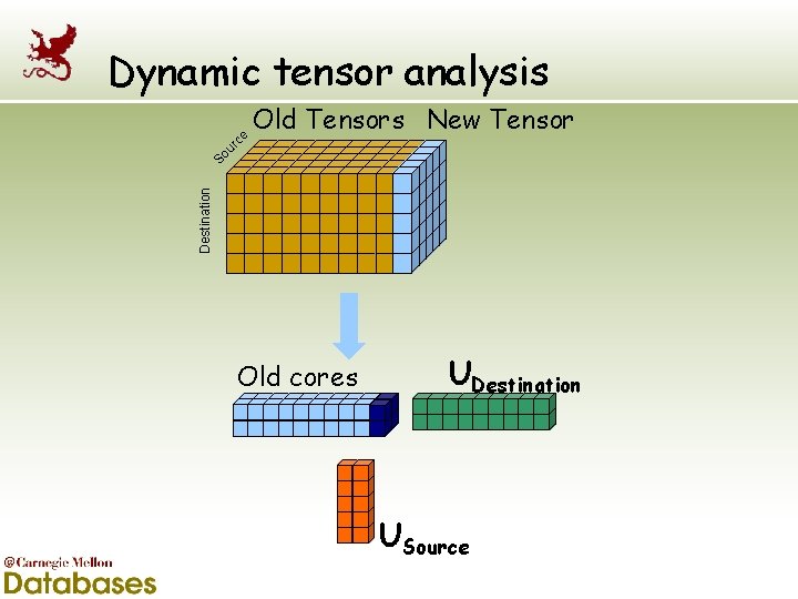
Old Tensors New Tensor Destination So ur ce Dynamic tensor analysis Old cores UDestination USource

Roadmap Motivation and main ideas Background and related work Dynamic and streaming tensor analysis Experiments Conclusion
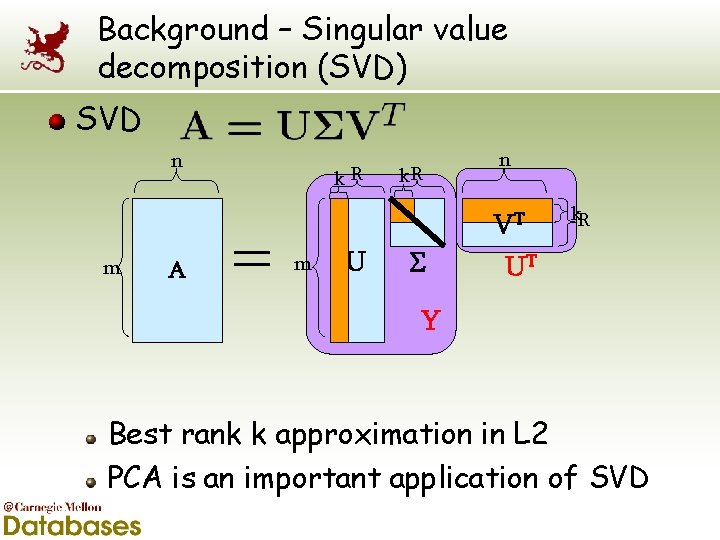
Background – Singular value decomposition (SVD) SVD n k. R n VT m A m U k. R UT Y Best rank k approximation in L 2 PCA is an important application of SVD
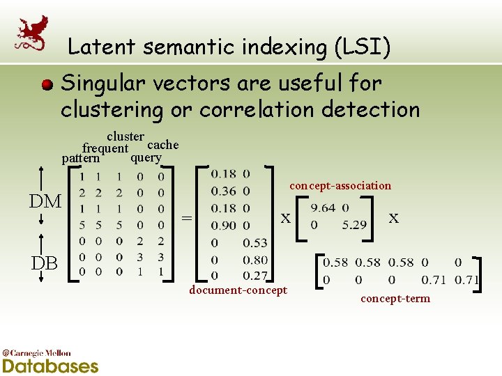
Latent semantic indexing (LSI) Singular vectors are useful for clustering or correlation detection cluster frequent cache query pattern DM concept-association = x x DB document-concept-term
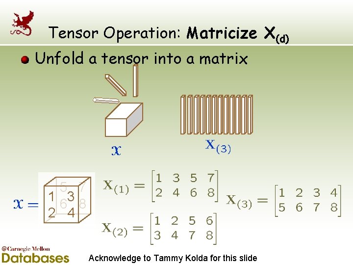
Tensor Operation: Matricize X(d) Unfold a tensor into a matrix 5 7 1 3 6 8 2 4 Acknowledge to Tammy Kolda for this slide
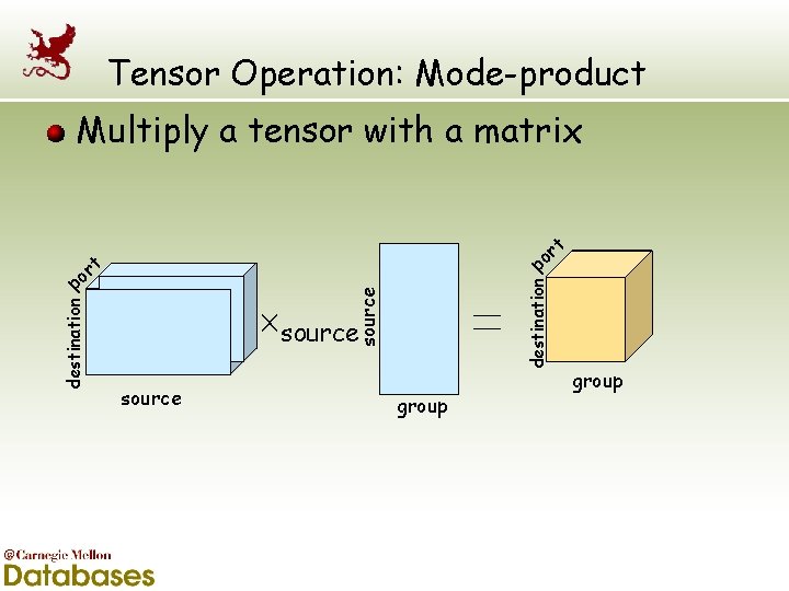
Tensor Operation: Mode-product Multiply a tensor with a matrix t r o p source destination t r po source group
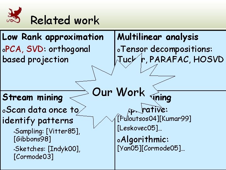
Related work Low Rank approximation o. PCA, SVD: orthogonal based projection Stream mining o. Scan data once to identify patterns Sampling: [Vitter 85], [Gibbons 98] • Sketches: [Indyk 00], [Cormode 03] • Multilinear analysis o. Tensor decompositions: Tucker, PARAFAC, HOSVD Our Work Graph mining o. Explorative: [Faloutsos 04][Kumar 99] [Leskovec 05]… o. Algorithmic: [Yan 05][Cormode 05]…
Roadmap Motivation and main ideas Background and related work Dynamic and streaming tensor analysis Experiments Conclusion
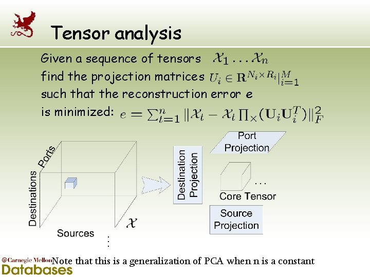
Tensor analysis Given a sequence of tensors find the projection matrices such that the reconstruction error e is minimized: … t … Note that this is a generalization of PCA when n is a constant
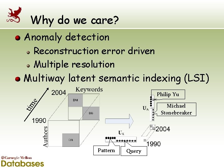
Why do we care? Anomaly detection Reconstruction error driven Multiple resolution Multiway latent semantic indexing (LSI) e Philip Yu tim Michael Stonebreaker Pattern Query
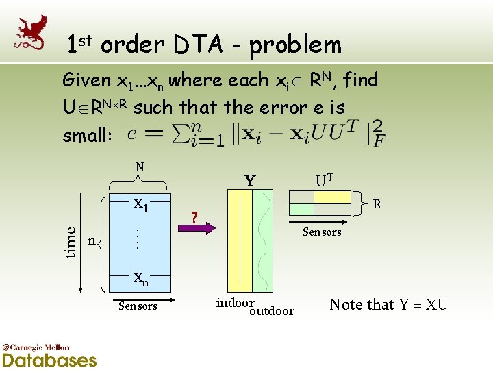
1 st order DTA - problem Given x 1…xn where each xi RN, find U RN R such that the error e is small: N n …. time x 1 Y UT R ? Sensors xn Sensors indoor outdoor Note that Y = XU
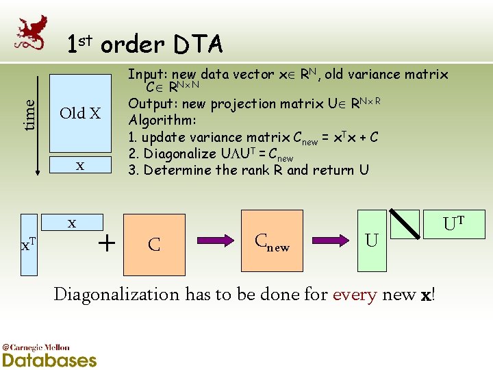
time 1 st order DTA Old X x x x. T Input: new data vector x RN, old variance matrix C RN N Output: new projection matrix U RN R Algorithm: 1. update variance matrix Cnew = x. Tx + C 2. Diagonalize U UT = Cnew 3. Determine the rank R and return U C Cnew U Diagonalization has to be done for every new x! UT
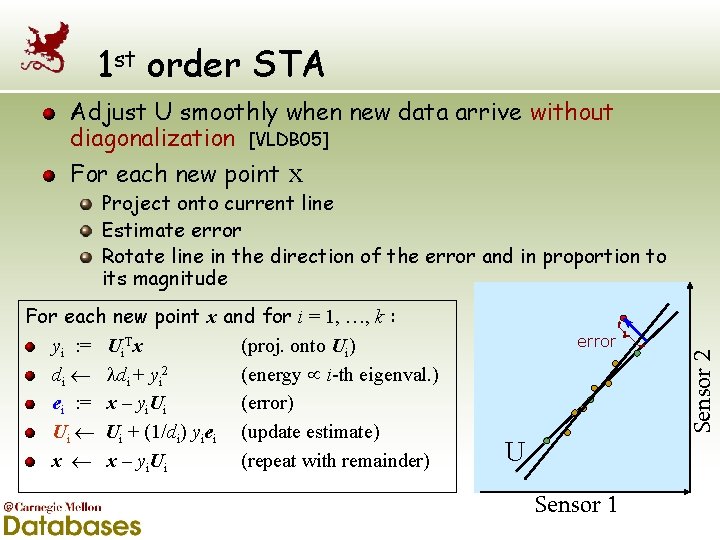
1 st order STA Adjust U smoothly when new data arrive without diagonalization [VLDB 05] For each new point x and for i = 1, …, k : yi : = Ui. Tx (proj. onto Ui) di + yi 2 (energy i-th eigenval. ) ei : = x – yi. Ui (error) Ui + (1/di) yiei (update estimate) x x – yi. Ui (repeat with remainder) error U Sensor 1 Sensor 2 Project onto current line Estimate error Rotate line in the direction of the error and in proportion to its magnitude
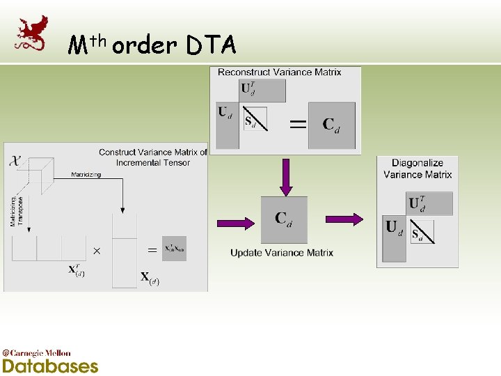
Mth order DTA
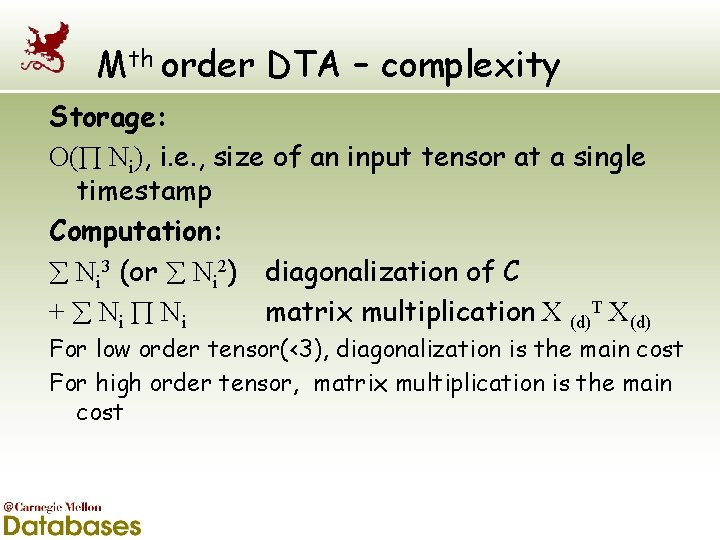
Mth order DTA – complexity Storage: O( Ni), i. e. , size of an input tensor at a single timestamp Computation: Ni 3 (or Ni 2) diagonalization of C + Ni matrix multiplication X (d)T X(d) For low order tensor(<3), diagonalization is the main cost For high order tensor, matrix multiplication is the main cost
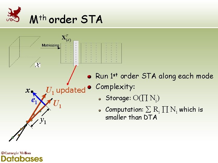
Mth order STA x e 1 U 1 updated U 1 y 1 Run 1 st order STA along each mode Complexity: O( Ni) Computation: Ri Ni which is Storage: smaller than DTA
Roadmap Motivation and main ideas Background and related work Dynamic and streaming tensor analysis Experiments Conclusion
Experiment Objectives Computational efficiency Accurate approximation Real applications § § Anomaly detection Clustering
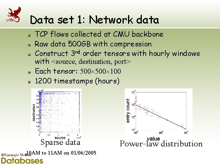
Data set 1: Network data TCP flows collected at CMU backbone Raw data 500 GB with compression Construct 3 rd order tensors with hourly windows with <source, destination, port> Each tensor: 500 100 1200 timestamps (hours) Sparse data 10 AM to 11 AM on 01/06/2005 value Power-law distribution
Data set 2: Bibliographic data (DBLP) Papers from VLDB and KDD conferences Construct 2 nd order tensors with yearly windows with <author, keywords> Each tensor: 4584 3741 11 timestamps (years)
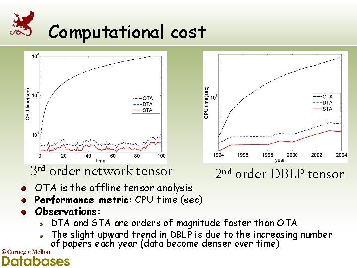
Computational cost 3 rd order network tensor OTA is the offline tensor analysis Performance metric: CPU time (sec) Observations: 2 nd order DBLP tensor DTA and STA are orders of magnitude faster than OTA The slight upward trend in DBLP is due to the increasing number of papers each year (data become denser over time)
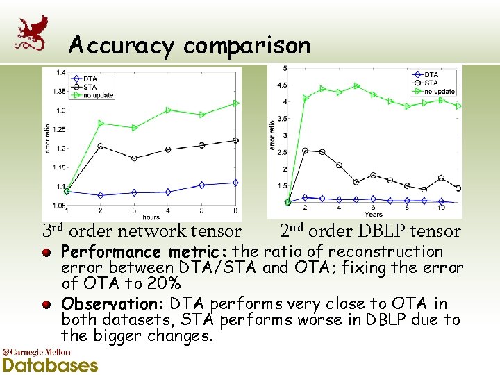
Accuracy comparison 3 rd order network tensor 2 nd order DBLP tensor Performance metric: the ratio of reconstruction error between DTA/STA and OTA; fixing the error of OTA to 20% Observation: DTA performs very close to OTA in both datasets, STA performs worse in DBLP due to the bigger changes.
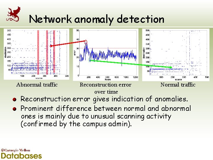
Network anomaly detection Abnormal traffic Reconstruction error over time Normal traffic Reconstruction error gives indication of anomalies. Prominent difference between normal and abnormal ones is mainly due to unusual scanning activity (confirmed by the campus admin).
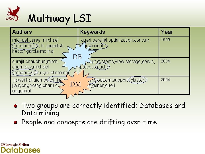
Multiway LSI Authors Keywords Year michael carey, michael stonebreaker, h. jagadish, hector garcia-molina queri, parallel, optimization, concurr, objectorient 1995 surajit chaudhuri, mitch cherniack, michael stonebreaker, ugur etintemel DB distribut, systems, view, storage, servic, process, cache jiawei han, jian pei, philip s. yu, streams, pattern, support, cluster, DMindex, gener, queri jianyong wang, charu c. aggarwal 2004 Two groups are correctly identified: Databases and Data mining People and concepts are drifting over time

Conclusion Tensor stream is a general data model DTA/STA incrementally decompose tensors into core tensors and projection matrices The result of DTA/STA can be used in other applications Anomaly detection Multiway LSI

Final word: Think structurally! The world is not flat, neither should data mining be. Contact: Jimeng Sun jimeng@cs. cmu. edu
- Slides: 34