Beyond Classical Search Chapter 4 Outline n Local

Beyond Classical Search Chapter 4

Outline n Local Greedy Search – Hill Climbing n Simulated Annealing n Genetic Algorithms

Local search algorithms n In many optimization problems, the path to the goal is irrelevant; the goal state itself is the solution n State space = set of "complete" configurations Find optimal configuration, e. g. , TSP n Find configuration satisfying constraints, e. g. , n -queens n n In such cases, we can use local search algorithms n keep a single "current" state, try to improve it n Constance space

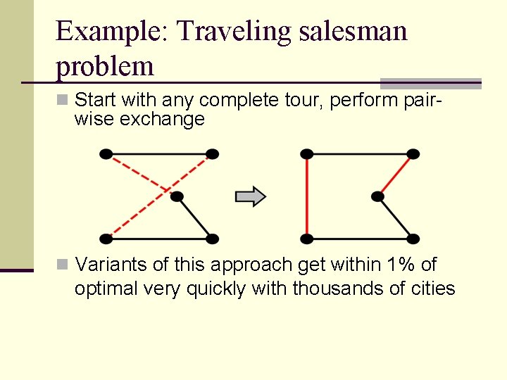
Example: Traveling salesman problem n Start with any complete tour, perform pair- wise exchange n Variants of this approach get within 1% of optimal very quickly with thousands of cities

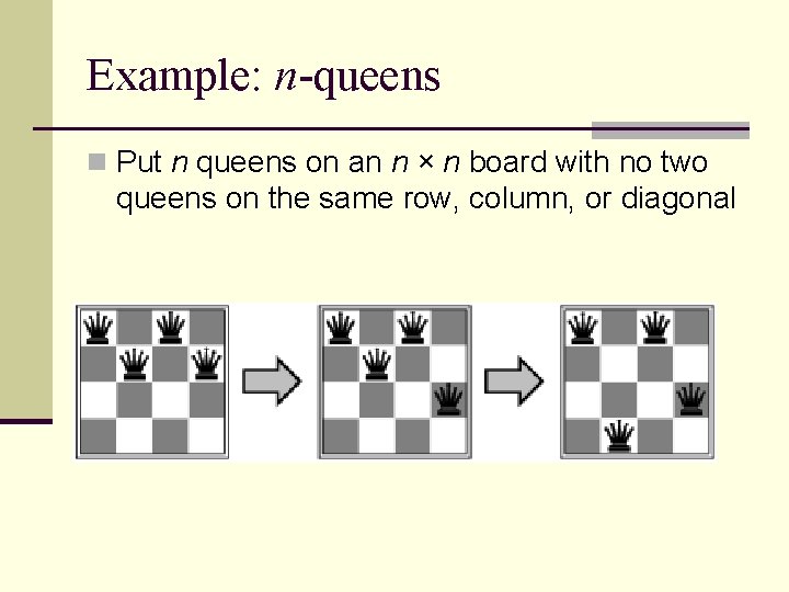
Example: n-queens n Put n queens on an n × n board with no two queens on the same row, column, or diagonal

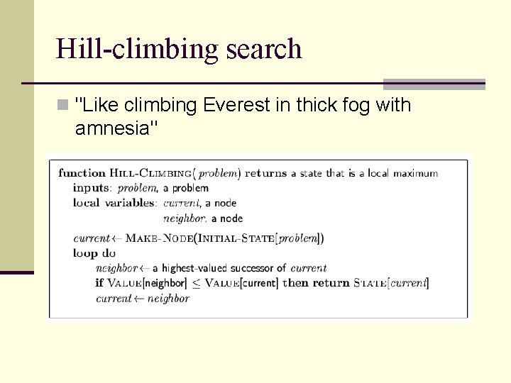
Hill-climbing search n "Like climbing Everest in thick fog with amnesia"

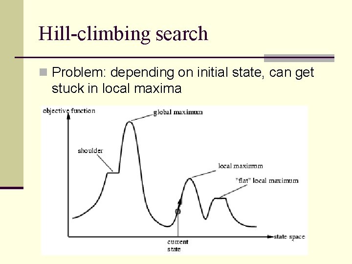
Hill-climbing search n Problem: depending on initial state, can get stuck in local maxima

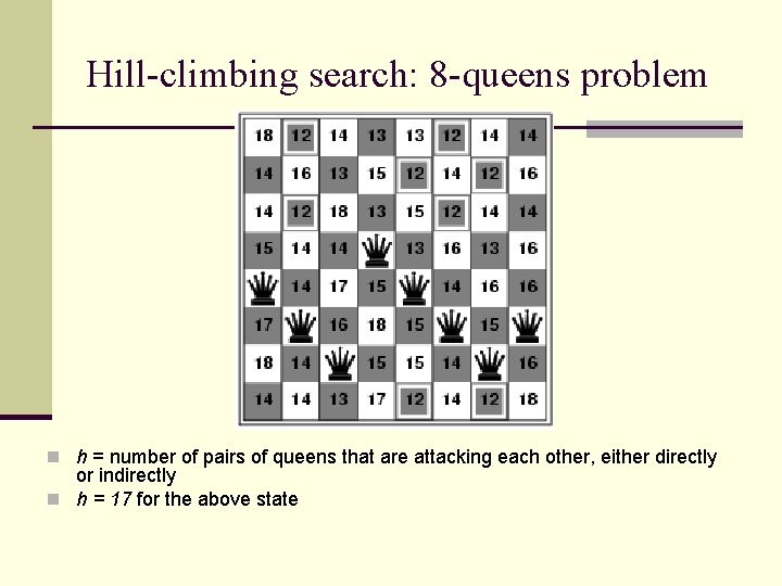
Hill-climbing search: 8 -queens problem n h = number of pairs of queens that are attacking each other, either directly or indirectly n h = 17 for the above state

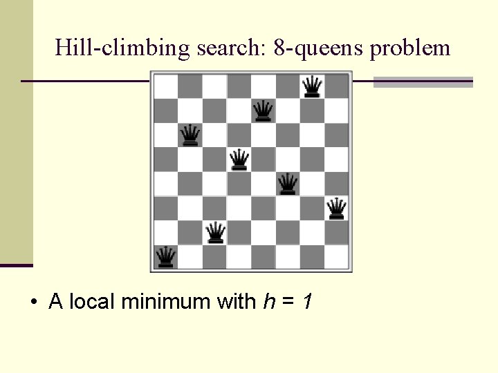
Hill-climbing search: 8 -queens problem • A local minimum with h = 1

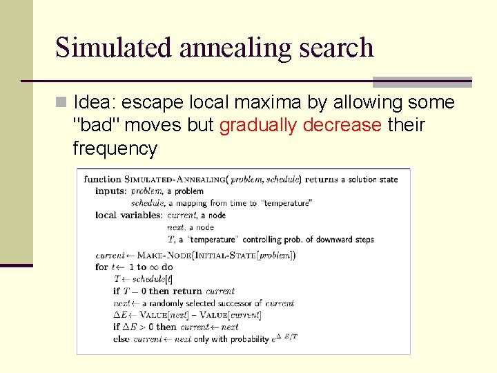
Simulated annealing search n Idea: escape local maxima by allowing some "bad" moves but gradually decrease their frequency

Properties of simulated annealing search n One can prove: If T decreases slowly enough, then simulated annealing search will find a global optimum with probability approaching 1 n Widely used in VLSI layout, airline scheduling, etc

Local beam search n Keep track of k states rather than just one n Start with k randomly generated states n At each iteration, all the successors of all k states are generated n If any one is a goal state, stop; else select the k best successors from the complete list and repeat.

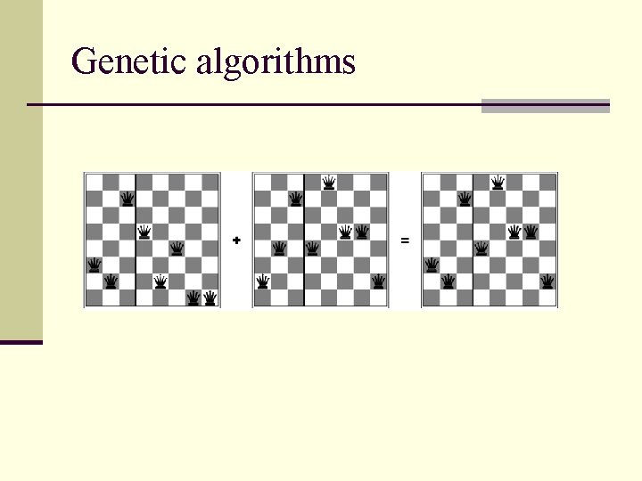
Genetic algorithms n A successor state is generated by combining two parent states n Start with k randomly generated states (population) n A state is represented as a string over a finite alphabet (often a string of 0 s and 1 s) n Evaluation function (fitness function). Higher values for better states. n Produce the next generation of states by selection, crossover, and mutation

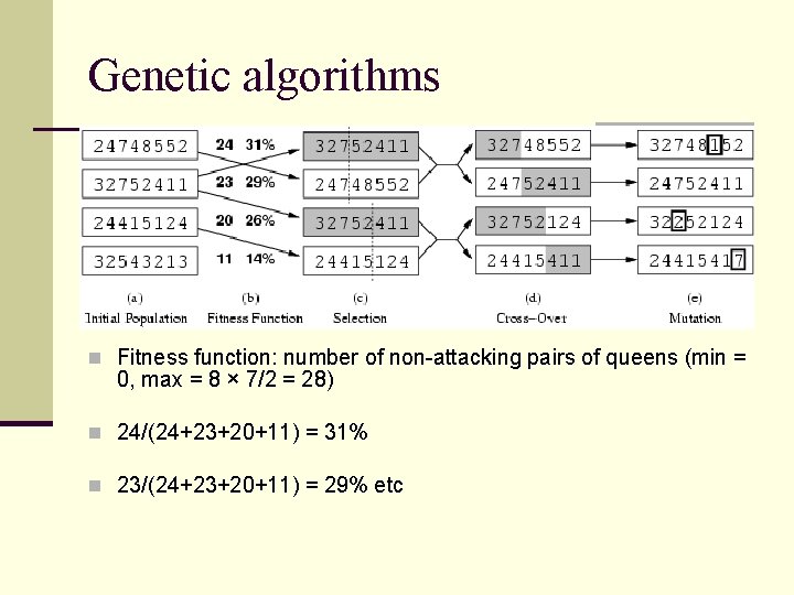
Genetic algorithms n Fitness function: number of non-attacking pairs of queens (min = 0, max = 8 × 7/2 = 28) n 24/(24+23+20+11) = 31% n 23/(24+23+20+11) = 29% etc

Genetic algorithms

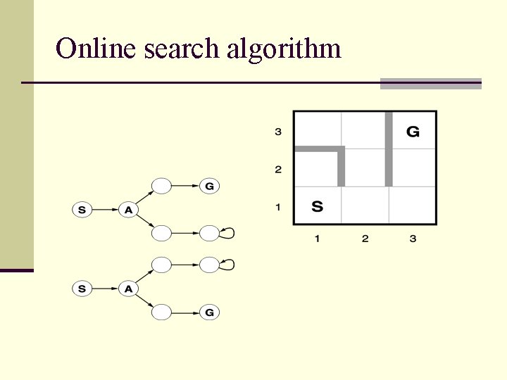
Online search algorithm n So far we talked about offline search n Compute a sequence of actions before taking an action n Online search interleaves action and computation n An online search agent knows: 1. 2. 3. Actions(s) Step cost function c(s, a, s’) Goal_test(s)

Online search algorithm

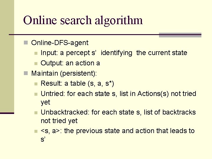
Online search algorithm n Online-DFS-agent Input: a percept s’ identifying the current state n Output: an action a n Maintain (persistent): n Result: a table (s, a, s*) n Untried: for each state s, list in Actions(s) not tried yet n Unbacktracked: for each state s, list of backtracks not tried yet n <s, a>: the previous state and action that leads to s’ n

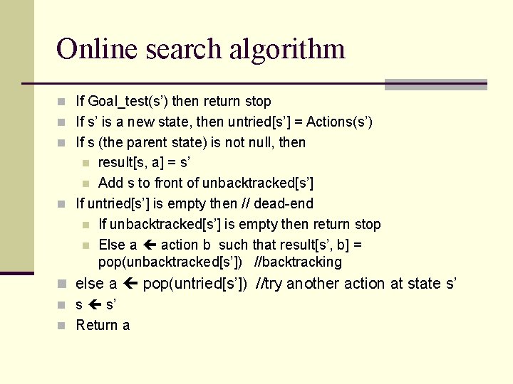
Online search algorithm n If Goal_test(s’) then return stop n If s’ is a new state, then untried[s’] = Actions(s’) n If s (the parent state) is not null, then result[s, a] = s’ n Add s to front of unbacktracked[s’] n If untried[s’] is empty then // dead-end n If unbacktracked[s’] is empty then return stop n Else a action b such that result[s’, b] = pop(unbacktracked[s’]) //backtracking n n else a pop(untried[s’]) //try another action at state s’ n s s’ n Return a

Summary n Local greedy search is efficient but not optimal - it can get stuck in a local optima n Simulated annealing uses randomized search controlled by “temperature” n Genetic Algorithm is a randomized search method patterned after natural evolution – “survival of the fittest”. n Search methods are often used for solving optimization problems such as TSP 20