Behavioural Finance Lecture 11 Part 2 Financial Instability

Behavioural Finance Lecture 11 Part 2 Financial Instability Hypothesis The Global Financial Crisis

Minsky’s “Financial Instability Hypothesis” • Essential point “it is necessary to have an economic theory which makes great depressions one of the possible states in which our type of capitalist economy can find itself. ” (Can "It” Happen Again? A Reprise) • Time-&-debt-aware model: – Economy in historical time – Debt-induced recession in recent past – Firms and banks conservative re debt/equity, assets – Only conservative projects are funded • Recovery means most projects succeed – Firms and banks revise risk premiums • Accepted debt/equity ratio rises • Assets revalued upwards…

The Euphoric Economy • Period of tranquility causes expectations to rise… – “Stability—or tranquility—in a world with a cyclical past and capitalist financial institutions is destabilizing. ” (The Financial Instability Hypothesis: A Restatement) • Self-fulfilling expectations – Decline in risk aversion causes increase in investment • Investment expansion causes economy to grow faster – Asset prices rise • speculation on assets profitable – Increased willingness to lend increases money supply • Money supply endogenous money, not under Fed control – Riskier investments enabled, asset speculation rises • The emergence of “Ponzi” financiers – Cash flow less than debt servicing costs – Profit by selling assets on rising market – Interest-rate insensitive demand for finance

The Assets Boom and Bust • Eventually: – Rising rates make conservative projects speculative – Non-Ponzi investors sell assets to service debts – Entry of new sellers floods asset markets – Rising trend of asset prices falters or reverses • Ponzi financiers go bankrupt: – Can no longer sell assets for a profit – Debt servicing on assets far exceeds cash flows • Asset prices collapse, increasing debt/equity ratios • Endogenous expansion of money supply reverses • Investment evaporates; economic growth slows • Economy enters a debt-induced recession – Back where we started. . .

Crisis and Aftermath • Low Inflation? – Debts cannot be repaid – Bankruptcies affect even non-speculative businesses – Economic activity remains suppressed: a Depression • Combination of falling output and deflation • High inflation – Rising nominal cash flows service debt – Inflation reduces debt to GDP ratio – “Stagflation”: low growth but moderate inflation

• Big Government? – Anti-cyclical spending and taxation of government enables debts to be repaid – Renewal of cycle once debt levels reduced – Stability is not avoidance of cycles, but avoidance of complete breakdown • Next: modelling FIH with Goodwin’s “growth cycle” model – based on Marx’s model of cycles in income distribution and employment:

Modelling Minsky & Endogenous Money… • Marx’s cyclical growth model in Capital I Ch. 25: – “a rise in the price of labor resulting from accumulation of capital implies. . . – accumulation slackens in consequence of the rise in the price of labour, because the stimulus of gain is blunted. – The rate of accumulation lessens; but with its lessening, the primary cause of that lessening vanishes, i. e. the disproportion between capital and exploitable labour power. – The mechanism of the process of capitalist production removes the very obstacles that it temporarily creates. – The price of labor falls again to a level corresponding with the needs of the self-expansion of capital, whether the level be below, the same as, or above the one which was normal before the rise of wages took place. . . ” (Marx 1867)

Modelling Minsky & Endogenous Money… • Marx’s model (1867) – High wages low investment low growth rising unemployment falling wage demands increased profit share rising investment high growth high employment High wages: cycle continues • Goodwin (1967) draws analogy with biology “predatorprey” models – Rate of growth of prey (fish = capitalists!) depends +ively on food supply and -ively interactions with predator (sharks = workers) – Rate of growth of predator depends -ively on number of predators and +ively on interactions with prey: • OK; now let’s build it. First, the maths…

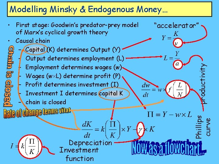
Modelling Minsky & Endogenous Money… Depreciation Investment function productivity “accelerator” Phillips curve • First stage: Goodwin’s predator-prey model of Marx’s cyclical growth theory • Causal chain – Capital (K) determines Output (Y) – Output determines employment (L) – Employment determines wages (w) – Wages (w L) determine profit (P) – Profit determines investment (I) – Investment I determines capital K – chain is closed

Modelling Minsky & Endogenous Money… • Capital K determines output Y via the accelerator: • Y determines employment L via productivity a: • L determines employment rate l via population N: • l determines rate of change of wages w via P. C. • (Linear Phillips curve for now) • Integral of w determines W (given initial value) • Y-W determines profits P and thus Investment I… • Closes the loop:

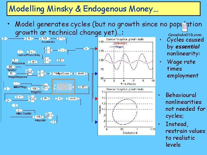
Modelling Minsky & Endogenous Money… • Model generates cycles (but no growth since no population growth or technical change yet)…: • Cycles caused by essential nonlinearity: • Wage rate times employment • Behavioural nonlinearities not needed for cycles; • Instead, restrain values to realistic levels

Modelling Minsky & Endogenous Money… • Let’s “do that again”, in stages – This time with • exponential growth in population & technology • Nonlinear Phillips curve • “Rates of change” first – The investment to capital relation is easy:

Modelling Minsky & Endogenous Money… • Next step is easy—output is capital stock divided by the accelerator: • Output divided by labour productivity gives the necessary employment level • Employment divided by the available workforce gives us the rate of employment • So we need a productivity component and a population component…

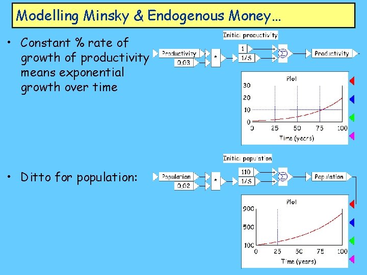
Modelling Minsky & Endogenous Money… • Constant % rate of growth of productivity means exponential growth over time • Ditto for population:

Modelling Minsky & Endogenous Money… • Output divided by labour productivity gives needed number of workers

Modelling Minsky & Endogenous Money… • Workforce divided by population gives rate of employment • Now things get a bit messy, so we hide bits we know about in compound blocks

Modelling Minsky & Endogenous Money… • The same model, with internal complexity simplified by compound blocks: • Now we need a wage change block—employment rate determines rate of change of wages • Wage change function more complicated because involves “Phillips curve” (Phillips researched the stats in the first place to build a model like this) • Next component is “generalised exponential function” set to reproduce same fit as Phillips curve

Modelling Minsky & Endogenous Money… • Feed in • minimum rate of change (-4%) • (x, y) coordinates for one point (. 96, 0) • Slope at this point (2) • And you get the exponential curve that fits these values: • In flowchart form, this is…

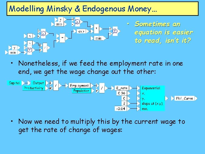
Modelling Minsky & Endogenous Money… • Sometimes an equation is easier to read, isn’t it? • Nonetheless, if we feed the employment rate in one end, we get the wage change out the other: • Now we need to multiply this by the current wage to get the rate of change of wages:

Modelling Minsky & Endogenous Money… • Wage change function: • So now the whole system is:

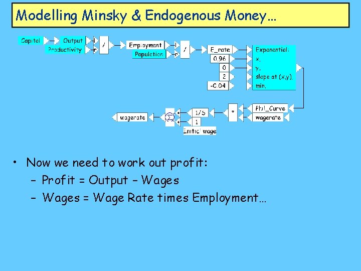
Modelling Minsky & Endogenous Money… • Now we need to work out profit: – Profit = Output – Wages = Wage Rate times Employment…

Modelling Minsky & Endogenous Money… • Since in the simple Goodwin model, capitalists invest all their profits, we simply need to link profit to capital (whose input is investment) and we have built the model:

Modelling Minsky & Endogenous Money… • Testing this out by adding some graphs; if it works, we should get cycles in the employment rate:

Modelling Minsky & Endogenous Money… • Voila! Now to tidy things up a bit using compound blocks…

Modelling Minsky & Endogenous Money… • Now at last we have the basis on which to build a Minsky model

Modelling Minsky & Endogenous Money… • Essential step to introduce Minsky/endogenous money is debt • For debt, essential that (at least) capitalists wish to invest more than they earn – “Debt seems to be the residual variable in financing decisions. Investment increases debt, and higher earnings tend to reduce debt. ” (Fama & French 1997) – “The source of financing most correlated with investment is long-term debt… These correlations confirm the impression that debt plays a key role in accommodating year-by-year variation in investment. ” (Fama & French 1998) • A nonlinear investment function needed for firms investment to be a function of rate of profit: Low— invest nothing; Medium—invest as much as earn; High—invest more than earn

Modelling Minsky & Endogenous Money… • Important (normal) feature of dynamic modelling: increasing generality of model makes it more realistic – No need for absurd assumptions to maintain fiction of equilibrium, coherent micro/macro behaviour • Use same exponential form as for Phillips, but with different parameters – Investment=Profit at profit rate of 3% – Investment>Profit at profit rate > 3% – Investment<Profit at profit rate < 3% – Slope of change at 3%=2 – Minimum investment – 1% output (depreciation easily introduced)

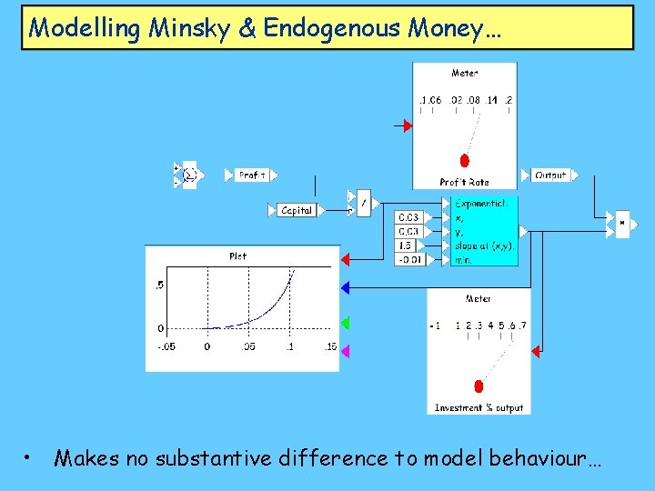
Modelling Minsky & Endogenous Money… • Makes no substantive difference to model behaviour…

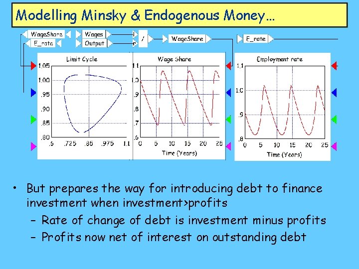
Modelling Minsky & Endogenous Money… • But prepares the way for introducing debt to finance investment when investment>profits – Rate of change of debt is investment minus profits – Profits now net of interest on outstanding debt

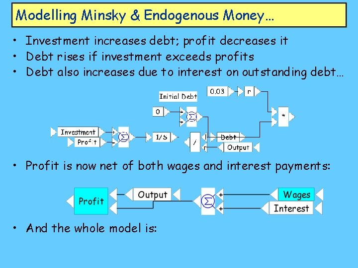
Modelling Minsky & Endogenous Money… • Investment increases debt; profit decreases it • Debt rises if investment exceeds profits • Debt also increases due to interest on outstanding debt… • Profit is now net of both wages and interest payments: • And the whole model is:

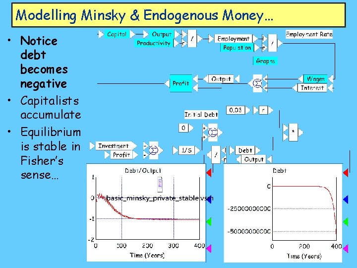
Modelling Minsky & Endogenous Money… • Notice debt becomes negative • Capitalists accumulate • Equilibrium is stable in Fisher’s sense…

Modelling Minsky & Endogenous Money… • “we may tentatively assume that, ordinarily and within wide limits, all, or almost all, economic variables tend, in a general way, towards a stable equilibrium” (Fisher 1933: 339) • BUT… – This stability of the kind Fisher describes: “so delicately poised that, after departure from it beyond certain limits, instability ensues” (Fisher 1933: 339). – Start further from equilibrium, and the system becomes unstable:

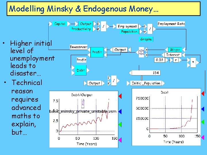
Modelling Minsky & Endogenous Money… • Higher initial level of unemployment leads to disaster… • Technical reason requires advanced maths to explain, but…

Modelling Minsky & Endogenous Money… • Technical reason is that nonlinear model can be – Locally stable around equilibrium (where “linear” component of system dominates) but – Globally unstable: past a certain range, higher power forces overwhelm linear component • Just as below one, a^3 is less than a^2 is less than a • But above 1, a^3 is bigger than a^2 is bigger than a – So if you start too far from equilibrium, you will suffer a debt-induced collapse – How do you get far from equilibrium? Tendency Minsky outlined for “euphoric expectations” to lead capitalists into excessive investment/optimism during a boom…

Modelling Minsky & Endogenous Money… • CAVEAT! – Dynamic modelling can capture many elements of Minsky’s theory and endogenous money, BUT – There are elements that cannot be modelled this way • Evolutionary change in the system • Non-systemic events—such as for example, people being persuaded by the failure of the system that the system must be changed – There is a limit to modelling—institutions and evolution and human agency must also be understood… – But we do at least get a better handle on the system by knowing its characteristic dynamics (even if we ignore that these characteristics can evolve…)

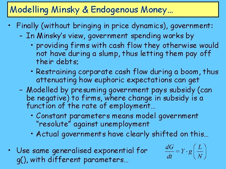
Modelling Minsky & Endogenous Money… • Finally (without bringing in price dynamics), government: – In Minsky’s view, government spending works by • providing firms with cash flow they otherwise would not have during a slump, thus letting them pay off their debts; • Restraining corporate cash flow during a boom, thus attenuating how euphoric expectations can get – Modelled by presuming government pays subsidy (can be negative) to firms, where change in subsidy is a function of the rate of employment… • Constant parameters means model government “resolute” against unemployment • Actual governments have clearly shifted on this… • Use same generalised exponential for g(), with different parameters…

Modelling Minsky & Endogenous Money… • Revised function gives negative exponential slope • Government – Keeps subsidy constant if unemployment=5% – Increases it gradually if U>5% – Reduces gradually if U<5% • Profit is now net of wages, interest, and government subsidy…

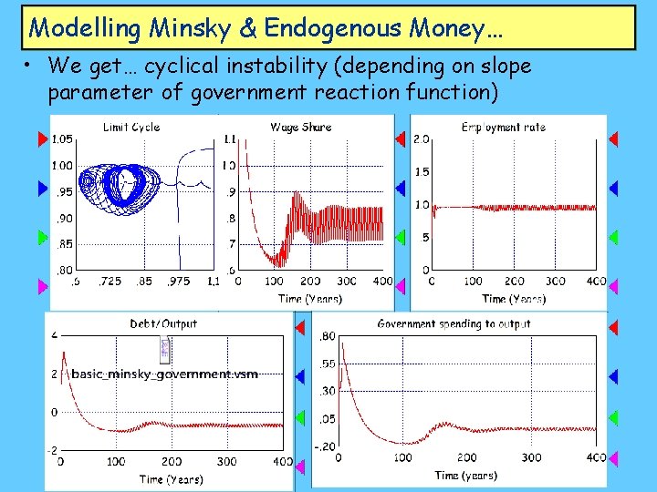
Modelling Minsky & Endogenous Money… • We get… cyclical instability (depending on slope parameter of government reaction function)

Modelling Minsky … Conclusion • Essentials of Financial Instability Hypothesis can be modelled using dynamic tools • Nuances of FIH require evolutionary perspective – Evolution of financial intermediaries over time… – Change in government policy… • Prices introduced in next lecture – Result is the “Fisher paradox” • Falling prices increase real debt burden even as actual debt levels reduced • Wrap up: main polemic weakness of debt-deflation hypothesis – (inability of Fisher, Keynes, Minsky to develop mathematical model)… • easily overcome with modern dynamic methods

Applying Minsky—the Global Financial Crisis • Knowledge of Minsky’s theory is why I predicted the GFC – Developed previous Minsky model in my Ph. D (1998) – Intended writing book-length version • Finance and Economic Breakdown (Edward Elgar Publishers) – Diverted to write Debunking Economics (Pluto Press & Zed Books 2001) • Disputes with neoclassicals occupied next 4 years – Late 2005, wrote Expert Witness report over predatory lending for NSW Legal Aid • Realised Debt/GDP on path to crisis • Predicted crisis in court testimony, March 2006

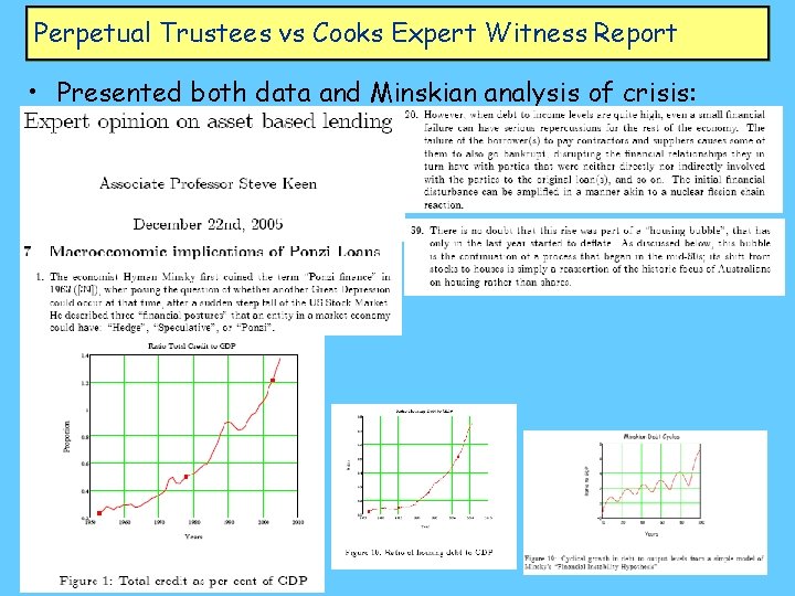
Perpetual Trustees vs Cooks Expert Witness Report • Presented both data and Minskian analysis of crisis:

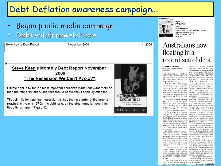
Debt Deflation awareness campaign. . . • Began public media campaign • Debtwatch newsletters

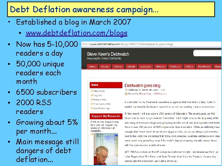
Debt Deflation awareness campaign. . . • Established a blog in March 2007 • www. debtdeflation. com/blogs • Now has 5 -10, 000 readers a day • 50, 000 unique readers each month • 6500 subscribers • 2000 RSS readers • Growing about 5% per month. . . • Main message still dangers of debt deflation. . .