Bayesian Support Vector Machine Classification Vasilis A Sotiris

Bayesian Support Vector Machine Classification Vasilis A. Sotiris AMSC 663 Midterm Presentation December 2007 University of Maryland College Park, MD 20783

Objectives • Develop an algorithm to detect anomalies in electronic systems (multivariate) • Improve detection sensitivity of classical Support Vector Machines (SVM) • Decrease false alarms • Predict future system performance

Methodology • Use linear Principal Component Analysis to decompose and compress raw data into two models: a) PCA model, and b) Residual model. • Use Support Vector Machines to classify data (in each model) into normal and abnormal classes • Assign probabilities to the classification output of the SVMs using a sigmoid function • Use a Maximum Likelihood Estimation to find the optimal sigmoid function parameters (in each model) • Determine the joint class probability from both models • Track changes to the joint probability to: – improve detection sensitivity – decrease false alarms – Predict future system performance

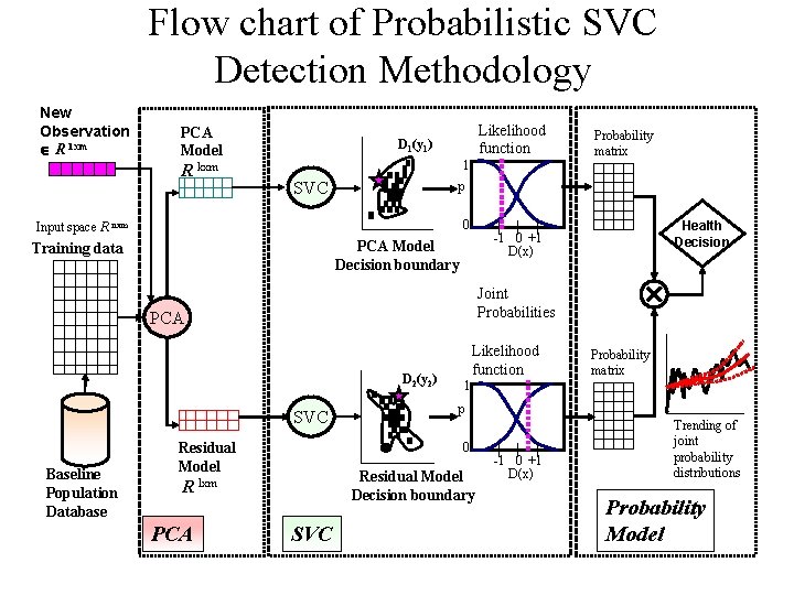
Flow chart of Probabilistic SVC Detection Methodology New Observation R 1 xm PCA Model R kxm Likelihood function D 1(y 1) 1 SVC p 0 Input space R nxm Joint Probabilities PCA Likelihood function D 2(y 2) SVC Baseline Population Database Residual Model p Residual Model Decision boundary SVC Probability matrix 1 0 R lxm PCA Health Decision -1 0 +1 D(x) PCA Model Decision boundary Training data Probability matrix -1 0 +1 D(x) Trending of joint probability distributions Probability Model

Principal Component Analysis

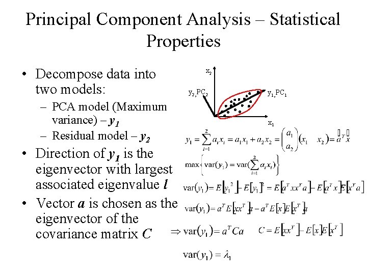
Principal Component Analysis – Statistical Properties • Decompose data into two models: – PCA model (Maximum variance) – y 1 – Residual model – y 2 • Direction of y 1 is the eigenvector with largest associated eigenvalue l • Vector a is chosen as the eigenvector of the covariance matrix C x 2 y 2, PC 2 y 1, PC 1 x 1

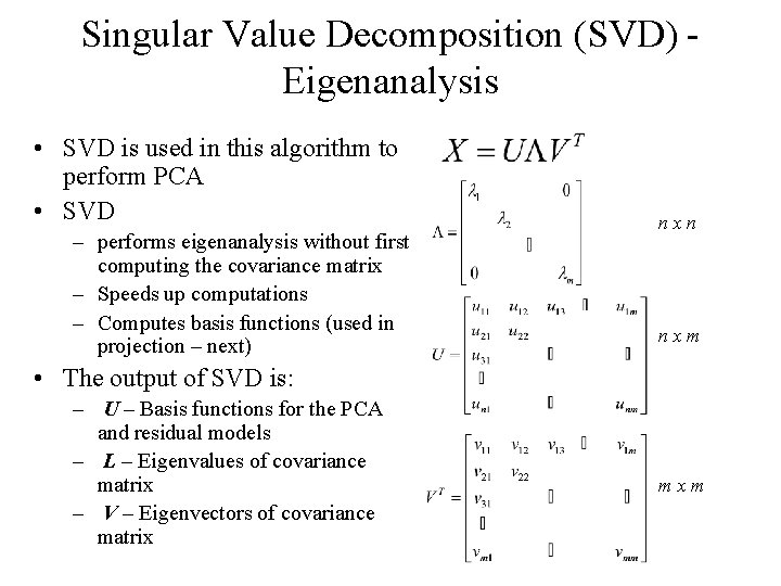
Singular Value Decomposition (SVD) Eigenanalysis • SVD is used in this algorithm to perform PCA • SVD – performs eigenanalysis without first computing the covariance matrix – Speeds up computations – Computes basis functions (used in projection – next) nxn nxm • The output of SVD is: – U – Basis functions for the PCA and residual models – L – Eigenvalues of covariance matrix – V – Eigenvectors of covariance matrix mxm

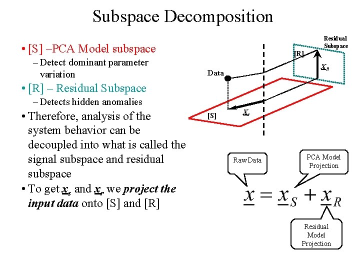
Subspace Decomposition Residual Subspace • [S] –PCA Model subspace – Detect dominant parameter variation [R] XR Data • [R] – Residual Subspace – Detects hidden anomalies • Therefore, analysis of the system behavior can be decoupled into what is called the signal subspace and residual subspace • To get xs and xr we project the input data onto [S] and [R] [S] Xs Raw Data PCA Model Projection Residual Model Projection

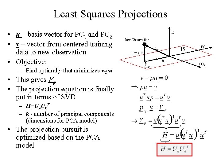
Least Squares Projections • u – basis vector for PC 1 and PC 2 • v – vector from centered training data to new observation • Objective: – Find optimal p that minimizes v-pu • This gives Vp • The projection equation is finally put in terms of SVD – H=Uk. T – k - number of principal components (dimensions for PCA model) • The projection pursuit is optimized based on the PCA model R New Observation [S] PC 1 PC 2

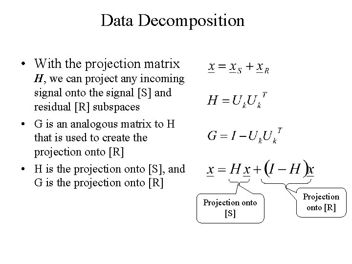
Data Decomposition • With the projection matrix H, we can project any incoming signal onto the signal [S] and residual [R] subspaces • G is an analogous matrix to H that is used to create the projection onto [R] • H is the projection onto [S], and G is the projection onto [R] Projection onto [S] Projection onto [R]

Support Vector Machines

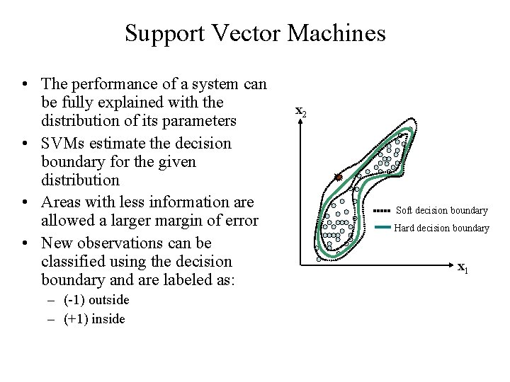
Support Vector Machines • The performance of a system can be fully explained with the distribution of its parameters • SVMs estimate the decision boundary for the given distribution • Areas with less information are allowed a larger margin of error • New observations can be classified using the decision boundary and are labeled as: – (-1) outside – (+1) inside x 2 Soft decision boundary Hard decision boundary x 1

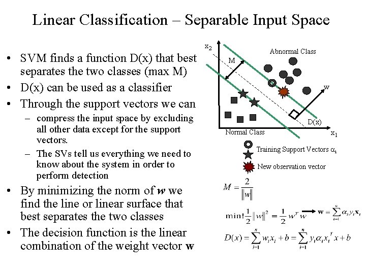
Linear Classification – Separable Input Space • SVM finds a function D(x) that best separates the two classes (max M) • D(x) can be used as a classifier • Through the support vectors we can – compress the input space by excluding all other data except for the support vectors. – The SVs tell us everything we need to know about the system in order to perform detection • By minimizing the norm of w we find the line or linear surface that best separates the two classes • The decision function is the linear combination of the weight vector w x 2 Abnormal Class M w D(x) Normal Class x 1 Training Support Vectors ai New observation vector

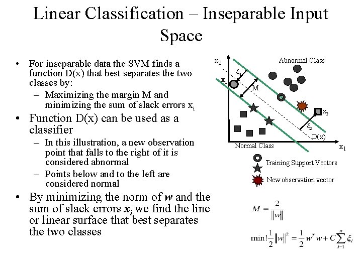
Linear Classification – Inseparable Input Space • For inseparable data the SVM finds a function D(x) that best separates the two classes by: – Maximizing the margin M and minimizing the sum of slack errors xi x 2 x 1 Abnormal Class x 1 M x 2 • Function D(x) can be used as a classifier – In this illustration, a new observation point that falls to the right of it is considered abnormal – Points below and to the left are considered normal • By minimizing the norm of w and the sum of slack errors xi we find the line or linear surface that best separates the two classes x 2 D(x) Normal Class Training Support Vectors New observation vector x 1

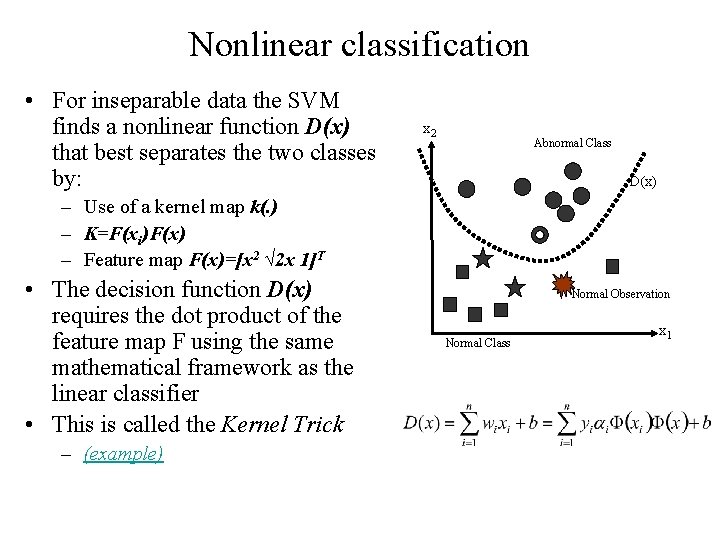
Nonlinear classification • For inseparable data the SVM finds a nonlinear function D(x) that best separates the two classes by: x 2 Abnormal Class D(x) – Use of a kernel map k(. ) – K=F(xi)F(x) – Feature map F(x)=[x 2 √ 2 x 1]T • The decision function D(x) requires the dot product of the feature map F using the same mathematical framework as the linear classifier • This is called the Kernel Trick – (example) Normal Observation Normal Class x 1

SVM Training

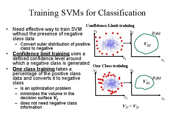
Training SVMs for Classification • Need effective way to train SVM without the presence of negative class data Confidence Limit training x 2 VS 1 – Convert outer distribution of positive class to negative • Confidence limit training uses a x 1 defined confidence level around which a negative class is generated One Class training • One class training takes a x 2 percentage of the positive class data and converts it to negative class – is an optimization problem – minimizes the volume in the decision surface VS – does not need negative class information D 1(x) x 1 x 2 x 1 VS 1 > VS 2 D 2(x) x 1

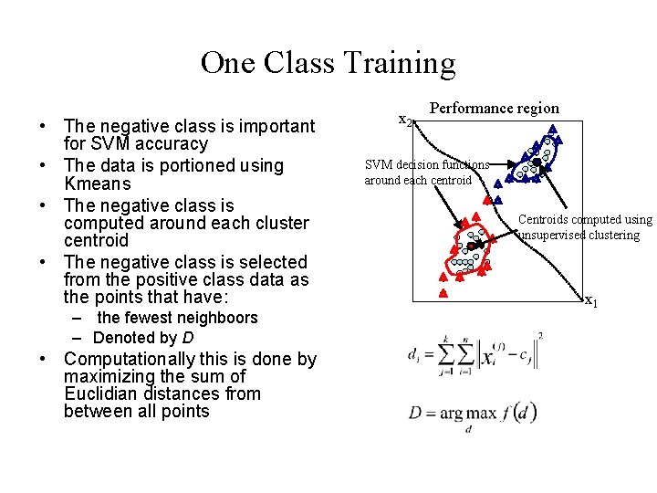
One Class Training • The negative class is important for SVM accuracy • The data is portioned using Kmeans • The negative class is computed around each cluster centroid • The negative class is selected from the positive class data as the points that have: – the fewest neighboors – Denoted by D • Computationally this is done by maximizing the sum of Euclidian distances from between all points x 2 Performance region SVM decision functions around each centroid Centroids computed using unsupervised clustering x 1

Class Prediction Probabilities and Maximum Likelihood Estimation

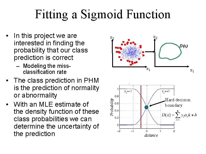
Fitting a Sigmoid Function • In this project we are interested in finding the probability that our class prediction is correct D(x) – Modeling the missclassification rate x 1 Hard decision boundary Probability • The class prediction in PHM is the prediction of normality or abnormality • With an MLE estimate of the density function of these class probabilities we can determine the uncertainty of the prediction x 2 distance

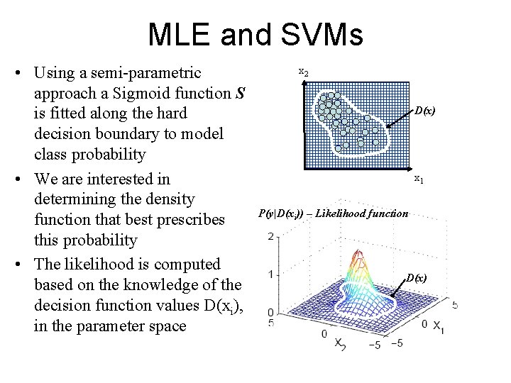
MLE and SVMs • Using a semi-parametric approach a Sigmoid function S is fitted along the hard decision boundary to model class probability • We are interested in determining the density function that best prescribes this probability • The likelihood is computed based on the knowledge of the decision function values D(xi), in the parameter space x 2 D(x) x 1 P(y|D(xi)) – Likelihood function D(x)

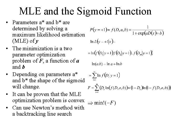
MLE and the Sigmoid Function • Parameters a* and b* are determined by solving a maximum likelihood estimation (MLE) of y • The minimization is a two parameter optimization problem of F, a function of a and b • Depending on parameters a* and b* the shape of the sigmoid will change. • It can be proven that the MLE optimization problem is convex • Can use Newton’s method with a backtracking line search

Joint Probability Model

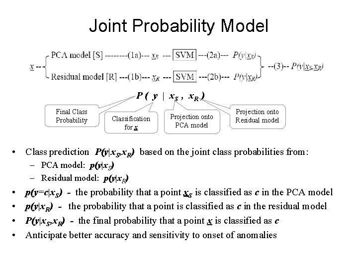
Joint Probability Model P ( y | x. S , x. R ) Final Class Probability Classification for x Projection onto PCA model Projection onto Residual model • Class prediction P(y|x. S, x. R) based on the joint class probabilities from: – PCA model: p(y|x. S) – Residual model: p(y|x. R) • • p(y=c|x. S) - the probability that a point x. S is classified as c in the PCA model p(y|x. R) - the probability that a point is classified as c in the residual model P(y|x. S, x. R) - the final probability that a point x is classified as c Anticipate better accuracy and sensitivity to onset of anomalies

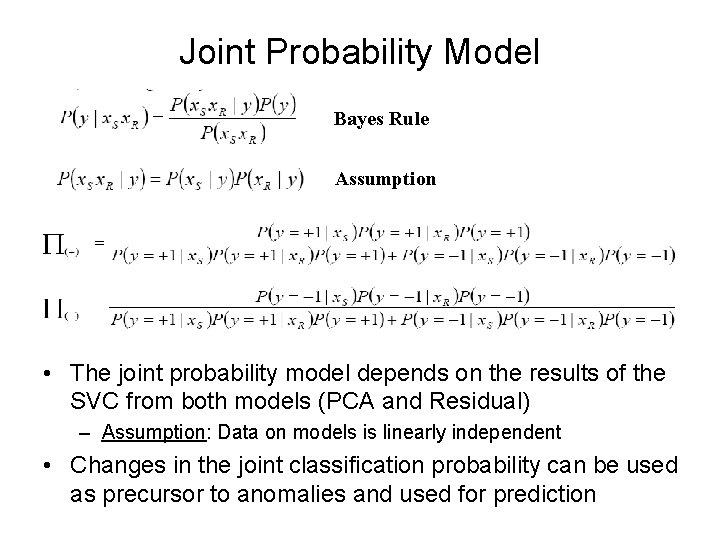
Joint Probability Model Bayes Rule Assumption • The joint probability model depends on the results of the SVC from both models (PCA and Residual) – Assumption: Data on models is linearly independent • Changes in the joint classification probability can be used as precursor to anomalies and used for prediction

Schedule/Progress

SVM Classification Example

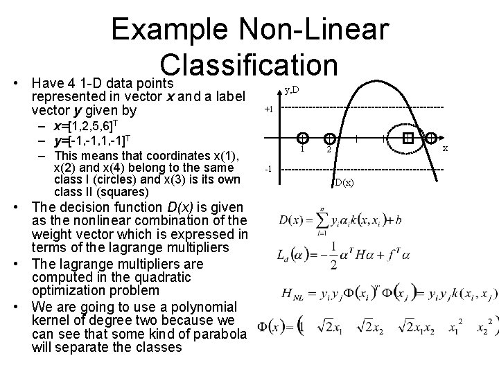
• Example Non-Linear Classification Have 4 1 -D data points represented in vector x and a label vector y given by – x=[1, 2, 5, 6]T – y=[-1, 1, -1]T – This means that coordinates x(1), x(2) and x(4) belong to the same class I (circles) and x(3) is its own class II (squares) • The decision function D(x) is given as the nonlinear combination of the weight vector which is expressed in terms of the lagrange multipliers • The lagrange multipliers are computed in the quadratic optimization problem • We are going to use a polynomial kernel of degree two because we can see that some kind of parabola will separate the classes y, D +1 1 x 2 -1 D(x)

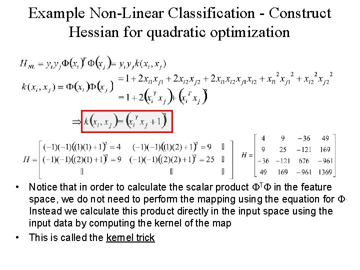
Example Non-Linear Classification - Construct Hessian for quadratic optimization • Notice that in order to calculate the scalar product FTF in the feature space, we do not need to perform the mapping using the equation for F. Instead we calculate this product directly in the input space using the input data by computing the kernel of the map • This is called the kernel trick

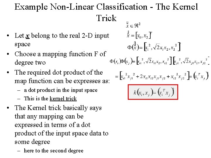
Example Non-Linear Classification - The Kernel Trick • Let x belong to the real 2 -D input space • Choose a mapping function F of degree two • The required dot product of the map function can be expresses as: – a dot product in the input space – This is the kernel trick • The Kernel trick basically says that any mapping can be expressed in terms of a dot product of the input space data to some degree – here to the second degree

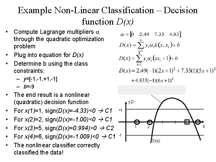
Example Non-Linear Classification – Decision function D(x) • Compute Lagrange multipliers a through the quadratic optimization problem • Plug into equation for D(x) • Determine b using the class constraints: – y=[-1, +1, -1] – b=-9 • The end result is a nonlinear (quadratic) decision function • For x(1)=1, sign(D(x)=-4. 33)<0 C 1 • For x(2)=2, sign(D(x)=-1. 00)<0 C 1 • For x(3)=5, sign(D(x)=0. 994)>0 C 2 • For x(4)=6, sign(D(x)=-1. 009)<0 C 1 • The nonlinear classifier correctly classified the data! y, D +1 1 x 2 -1 D(x)

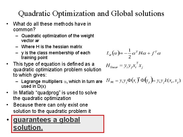
Quadratic Optimization and Global solutions • What do all these methods have in common? – Quadratic optimization of the weight vector w – Where H is the hessian matrix – y is the class membership of each training point • This type of equation is defined as a quadratic optimization problem solution to which gives: – Lagrange multipliers a, which in turn are used in D(x) • In Matlab “quadprog” is used to solve the quadratic optimization • Because there can only exist one solution to the quadratic problem it • guarantees a global solution.