Bayesian Networks Read RN Ch 14 1 14

Bayesian Networks Read R&N Ch. 14. 1 -14. 2 Next lecture: Read R&N 18. 1 -18. 4

You will be expected to know • Basic concepts and vocabulary of Bayesian networks. – Nodes represent random variables. – Directed arcs represent (informally) direct influences. – Conditional probability tables, P( Xi | Parents(Xi) ). • Given a Bayesian network: – Write down the full joint distribution it represents. • Given a full joint distribution in factored form: – Draw the Bayesian network that represents it. • Given a variable ordering and some background assertions of conditional independence among the variables: – Write down the factored form of the full joint distribution, as simplified by the conditional independence assertions.

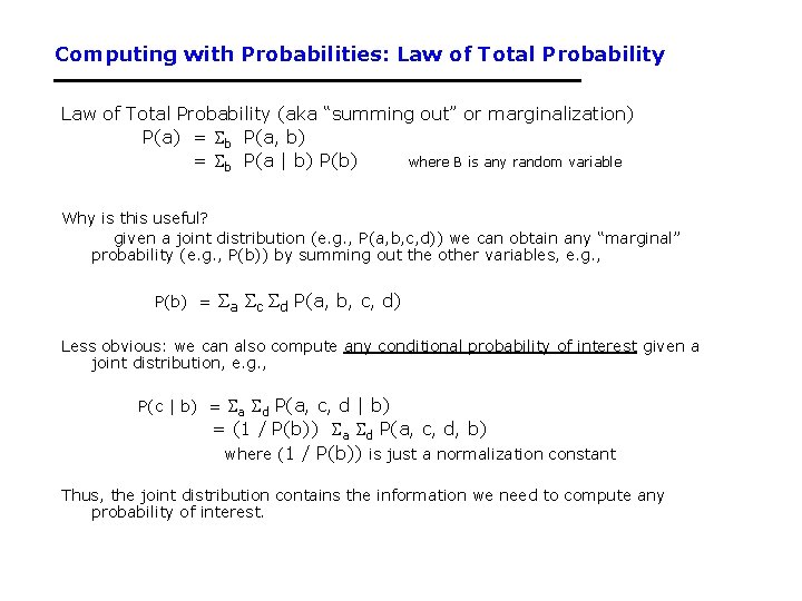
Computing with Probabilities: Law of Total Probability (aka “summing out” or marginalization) P(a) = b P(a, b) = b P(a | b) P(b) where B is any random variable Why is this useful? given a joint distribution (e. g. , P(a, b, c, d)) we can obtain any “marginal” probability (e. g. , P(b)) by summing out the other variables, e. g. , P(b) = a c d P(a, b, c, d) Less obvious: we can also compute any conditional probability of interest given a joint distribution, e. g. , P(c | b) = a d P(a, c, d | b) = (1 / P(b)) a d P(a, c, d, b) where (1 / P(b)) is just a normalization constant Thus, the joint distribution contains the information we need to compute any probability of interest.

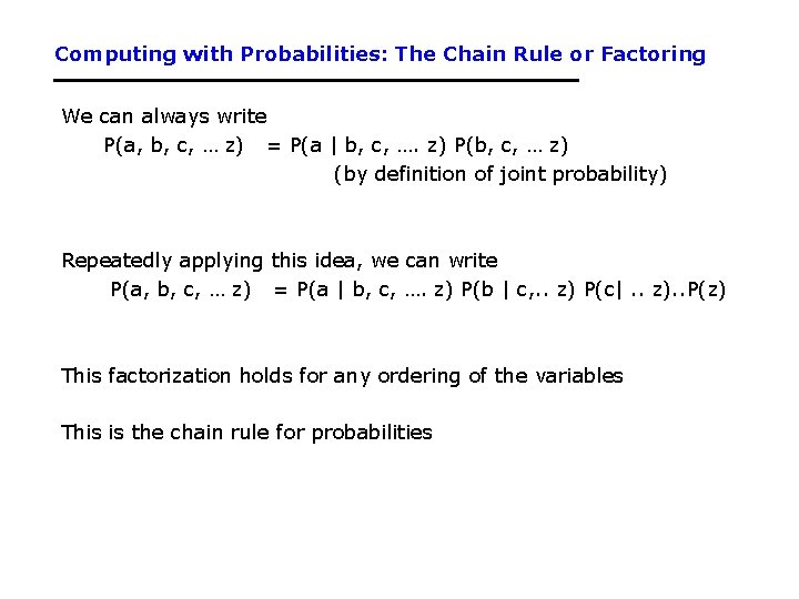
Computing with Probabilities: The Chain Rule or Factoring We can always write P(a, b, c, … z) = P(a | b, c, …. z) P(b, c, … z) (by definition of joint probability) Repeatedly applying this idea, we can write P(a, b, c, … z) = P(a | b, c, …. z) P(b | c, . . z) P(c|. . z). . P(z) This factorization holds for any ordering of the variables This is the chain rule for probabilities

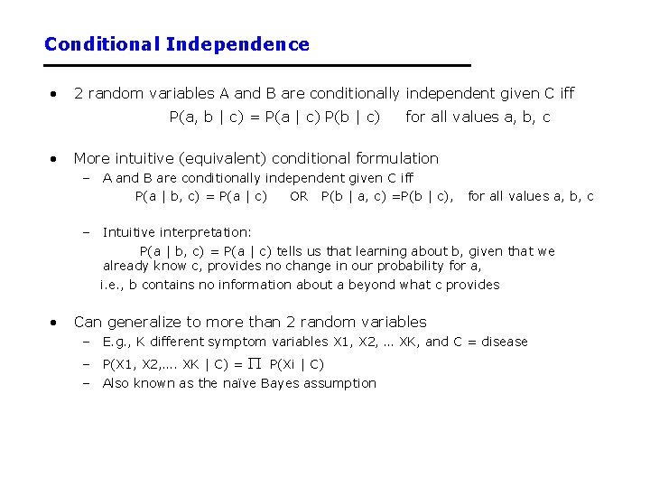
Conditional Independence • 2 random variables A and B are conditionally independent given C iff P(a, b | c) = P(a | c) P(b | c) • for all values a, b, c More intuitive (equivalent) conditional formulation – A and B are conditionally independent given C iff P(a | b, c) = P(a | c) OR P(b | a, c) =P(b | c), for all values a, b, c – Intuitive interpretation: P(a | b, c) = P(a | c) tells us that learning about b, given that we already know c, provides no change in our probability for a, i. e. , b contains no information about a beyond what c provides • Can generalize to more than 2 random variables – E. g. , K different symptom variables X 1, X 2, … XK, and C = disease – P(X 1, X 2, …. XK | C) = P(Xi | C) – Also known as the naïve Bayes assumption

“…probability theory is more fundamentally concerned with the structure of reasoning and causation than with numbers. ” Glenn Shafer and Judea Pearl Introduction to Readings in Uncertain Reasoning, Morgan Kaufmann, 1990

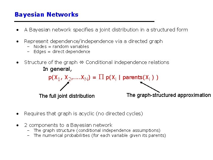
Bayesian Networks • A Bayesian network specifies a joint distribution in a structured form • Represent dependence/independence via a directed graph • Structure of the graph Conditional independence relations – Nodes = random variables – Edges = direct dependence In general, p(X 1, X 2, . . XN) = p(Xi | parents(Xi ) ) The full joint distribution The graph-structured approximation • Requires that graph is acyclic (no directed cycles) • 2 components to a Bayesian network – The graph structure (conditional independence assumptions) – The numerical probabilities (for each variable given its parents)

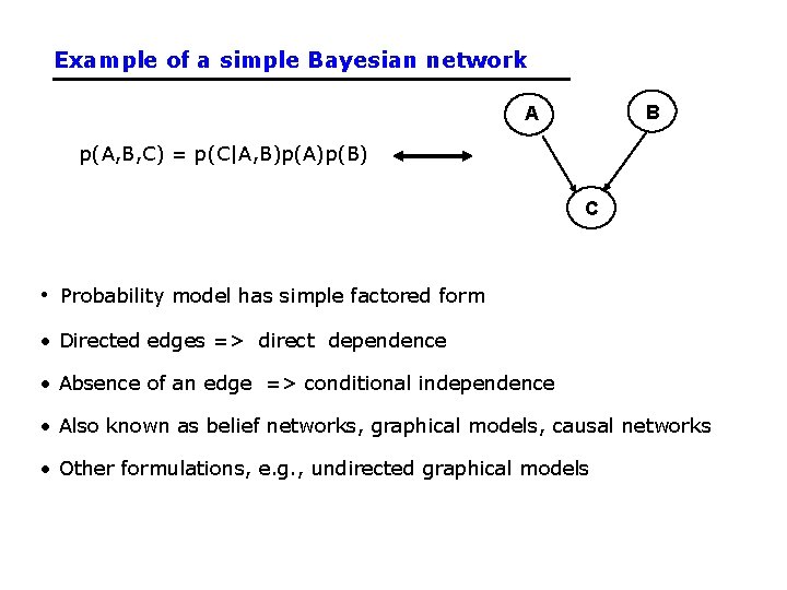
Example of a simple Bayesian network B A p(A, B, C) = p(C|A, B)p(A)p(B) C • Probability model has simple factored form • Directed edges => direct dependence • Absence of an edge => conditional independence • Also known as belief networks, graphical models, causal networks • Other formulations, e. g. , undirected graphical models

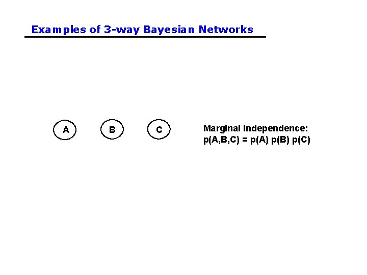
Examples of 3 -way Bayesian Networks A B C Marginal Independence: p(A, B, C) = p(A) p(B) p(C)

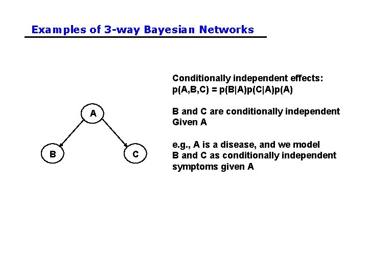
Examples of 3 -way Bayesian Networks Conditionally independent effects: p(A, B, C) = p(B|A)p(C|A)p(A) B and C are conditionally independent Given A A B C e. g. , A is a disease, and we model B and C as conditionally independent symptoms given A

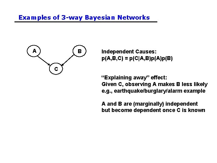
Examples of 3 -way Bayesian Networks A B Independent Causes: p(A, B, C) = p(C|A, B)p(A)p(B) C “Explaining away” effect: Given C, observing A makes B less likely e. g. , earthquake/burglary/alarm example A and B are (marginally) independent but become dependent once C is known

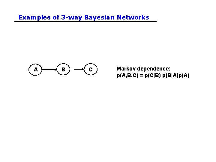
Examples of 3 -way Bayesian Networks A B C Markov dependence: p(A, B, C) = p(C|B) p(B|A)p(A)

Example • Consider the following 5 binary variables: – – – B = a burglary occurs at your house E = an earthquake occurs at your house A = the alarm goes off J = John calls to report the alarm M = Mary calls to report the alarm – What is P(B | M, J) ? (for example) – We can use the full joint distribution to answer this question • Requires 25 = 32 probabilities • Can we use prior domain knowledge to come up with a Bayesian network that requires fewer probabilities?

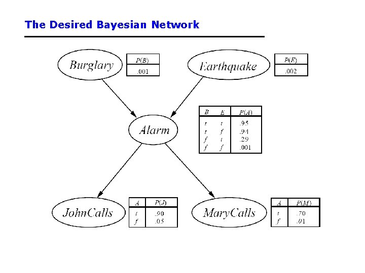
The Desired Bayesian Network

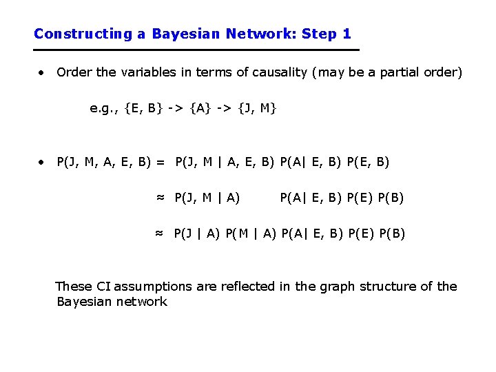
Constructing a Bayesian Network: Step 1 • Order the variables in terms of causality (may be a partial order) e. g. , {E, B} -> {A} -> {J, M} • P(J, M, A, E, B) = P(J, M | A, E, B) P(A| E, B) P(E, B) ≈ P(J, M | A) P(A| E, B) P(E) P(B) ≈ P(J | A) P(M | A) P(A| E, B) P(E) P(B) These CI assumptions are reflected in the graph structure of the Bayesian network

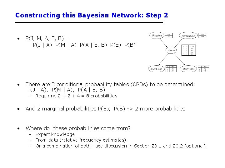
Constructing this Bayesian Network: Step 2 • P(J, M, A, E, B) = P(J | A) P(M | A) P(A | E, B) P(E) P(B) • There are 3 conditional probability tables (CPDs) to be determined: P(J | A), P(M | A), P(A | E, B) – Requiring 2 + 4 = 8 probabilities • And 2 marginal probabilities P(E), P(B) -> 2 more probabilities • Where do these probabilities come from? – Expert knowledge – From data (relative frequency estimates) – Or a combination of both - see discussion in Section 20. 1 and 20. 2 (optional)

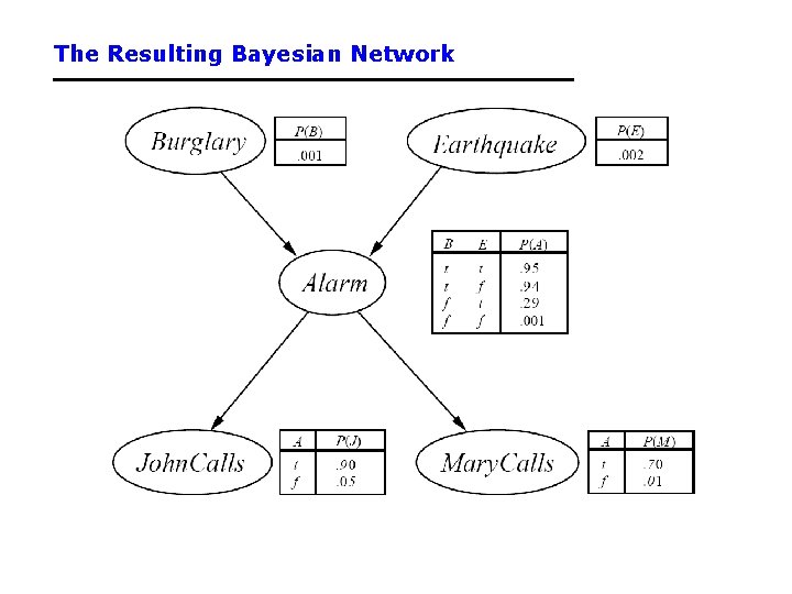
The Resulting Bayesian Network

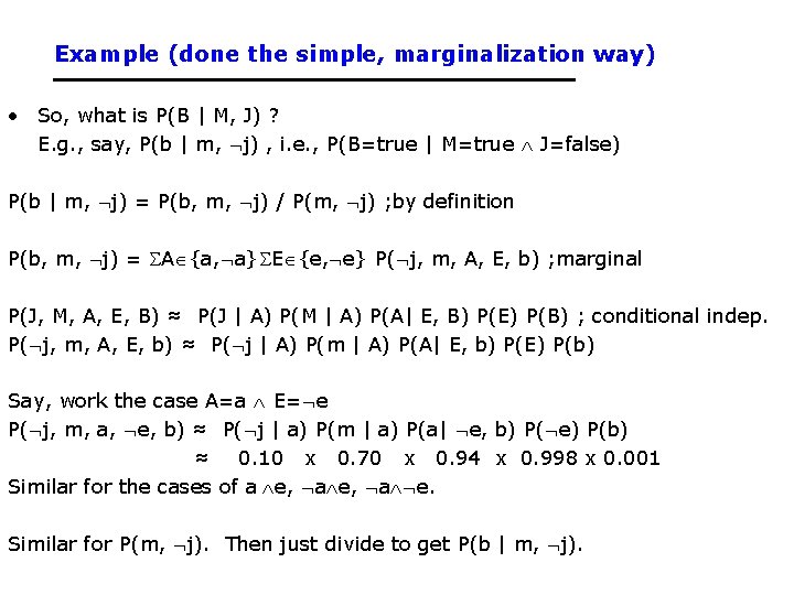
Example (done the simple, marginalization way) • So, what is P(B | M, J) ? E. g. , say, P(b | m, j) , i. e. , P(B=true | M=true J=false) P(b | m, j) = P(b, m, j) / P(m, j) ; by definition P(b, m, j) = A {a, a} E {e, e} P( j, m, A, E, b) ; marginal P(J, M, A, E, B) ≈ P(J | A) P(M | A) P(A| E, B) P(E) P(B) ; conditional indep. P( j, m, A, E, b) ≈ P( j | A) P(m | A) P(A| E, b) P(E) P(b) Say, work the case A=a E= e P( j, m, a, e, b) ≈ P( j | a) P(m | a) P(a| e, b) P( e) P(b) ≈ 0. 10 x 0. 70 x 0. 94 x 0. 998 x 0. 001 Similar for the cases of a e, a e. Similar for P(m, j). Then just divide to get P(b | m, j).

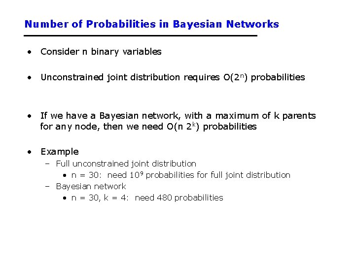
Number of Probabilities in Bayesian Networks • Consider n binary variables • Unconstrained joint distribution requires O(2 n) probabilities • If we have a Bayesian network, with a maximum of k parents for any node, then we need O(n 2 k) probabilities • Example – Full unconstrained joint distribution • n = 30: need 109 probabilities for full joint distribution – Bayesian network • n = 30, k = 4: need 480 probabilities

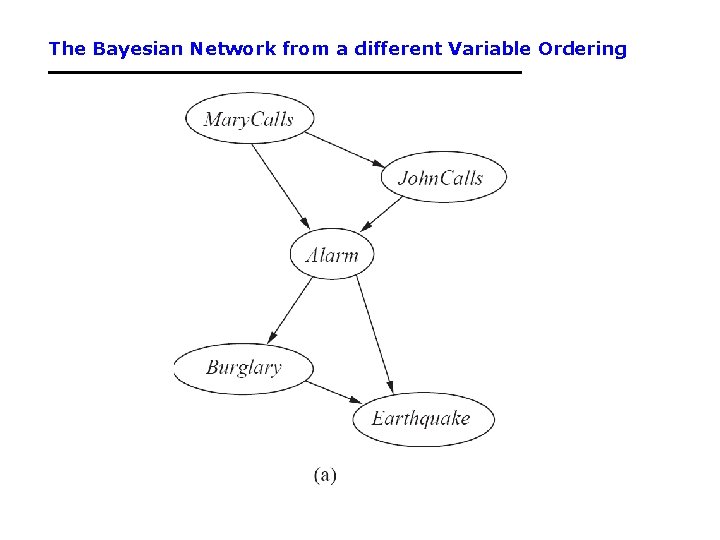
The Bayesian Network from a different Variable Ordering

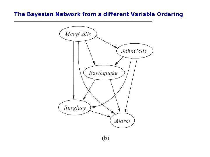
The Bayesian Network from a different Variable Ordering

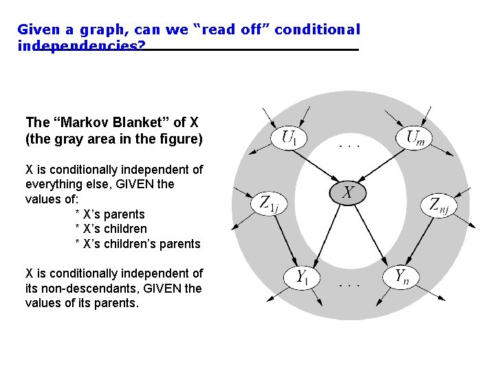
Given a graph, can we “read off” conditional independencies? The “Markov Blanket” of X (the gray area in the figure) X is conditionally independent of everything else, GIVEN the values of: * X’s parents * X’s children’s parents X is conditionally independent of its non-descendants, GIVEN the values of its parents.

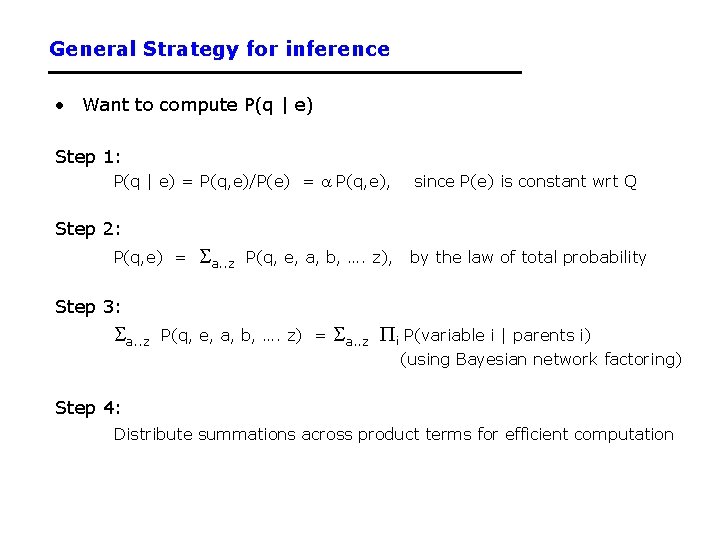
General Strategy for inference • Want to compute P(q | e) Step 1: P(q | e) = P(q, e)/P(e) = a P(q, e), since P(e) is constant wrt Q Step 2: P(q, e) = a. . z P(q, e, a, b, …. z), by the law of total probability Step 3: a. . z P(q, e, a, b, …. z) = a. . z i P(variable i | parents i) (using Bayesian network factoring) Step 4: Distribute summations across product terms for efficient computation

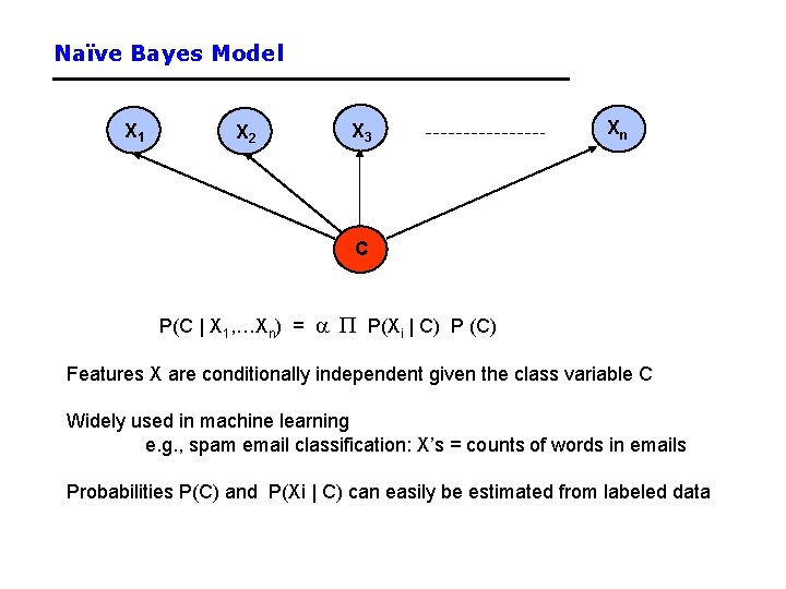
Naïve Bayes Model X 1 X 2 X 3 Xn C P(C | X 1, …Xn) = a P(Xi | C) P (C) Features X are conditionally independent given the class variable C Widely used in machine learning e. g. , spam email classification: X’s = counts of words in emails Probabilities P(C) and P(Xi | C) can easily be estimated from labeled data

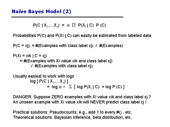
Naïve Bayes Model (2) P(C | X 1, …Xn) = a P(Xi | C) P (C) Probabilities P(C) and P(Xi | C) can easily be estimated from labeled data P(C = cj) ≈ #(Examples with class label cj) / #(Examples) P(Xi = xik | C = cj) ≈ #(Examples with Xi value xik and class label cj) / #(Examples with class label cj) Usually easiest to work with logs log [ P(C | X 1, …Xn) ] = log a + [ log P(Xi | C) + log P (C) ] DANGER: Suppose ZERO examples with Xi value xik and class label cj ? An unseen example with Xi value xik will NEVER predict class label cj ! Practical solutions: Pseudocounts, e. g. , add 1 to every #() , etc. Theoretical solutions: Bayesian inference, beta distribution, etc.

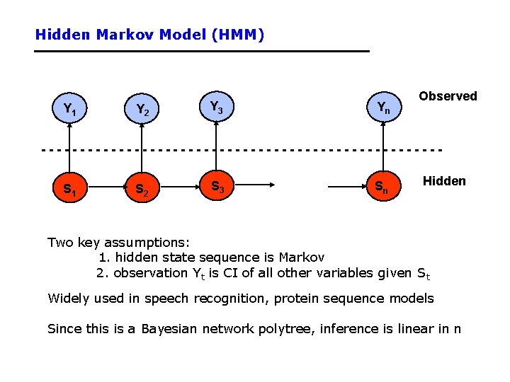
Hidden Markov Model (HMM) Y 1 Y 2 Y 3 Yn Observed --------------------------S 1 S 2 S 3 Sn Hidden Two key assumptions: 1. hidden state sequence is Markov 2. observation Yt is CI of all other variables given St Widely used in speech recognition, protein sequence models Since this is a Bayesian network polytree, inference is linear in n

Summary • Bayesian networks represent a joint distribution using a graph • The graph encodes a set of conditional independence assumptions • Answering queries (or inference or reasoning) in a Bayesian network amounts to efficient computation of appropriate conditional probabilities • Probabilistic inference is intractable in the general case – But can be carried out in linear time for certain classes of Bayesian networks