Bayesian modelling of differential gene expression data Sylvia

Bayesian modelling of differential gene expression data Sylvia Richardson, with Alex Lewin Department of Epidemiology and Public Health, Imperial College In collaboration with Anne Mette Hein and Clare Marshall (Imperial) Philippe Broët (INSERM) and Peter Green (Bristol) Helen Causton and Tim Aitman (Hammersmith)

Outline • Introduction: what is gene expression data ? • Array effects (normalisation) • Exchangeable model for the gene specific variances and Bayesian model checks • Differential expression • Rank statistics • Mixture models for differential expression

What is gene expression data ? Protein-encoding genes are transcribed into m. RNA (messenger), and the m. RNA is translated to make proteins, the building blocks of living cells DNA Microarrays can be used to measure the relative abundance of m. RNA, providing information on gene expression in a particular cell type, under particular conditions The fundamental principle used to measure the expression is that of hybridisation Introduction 1

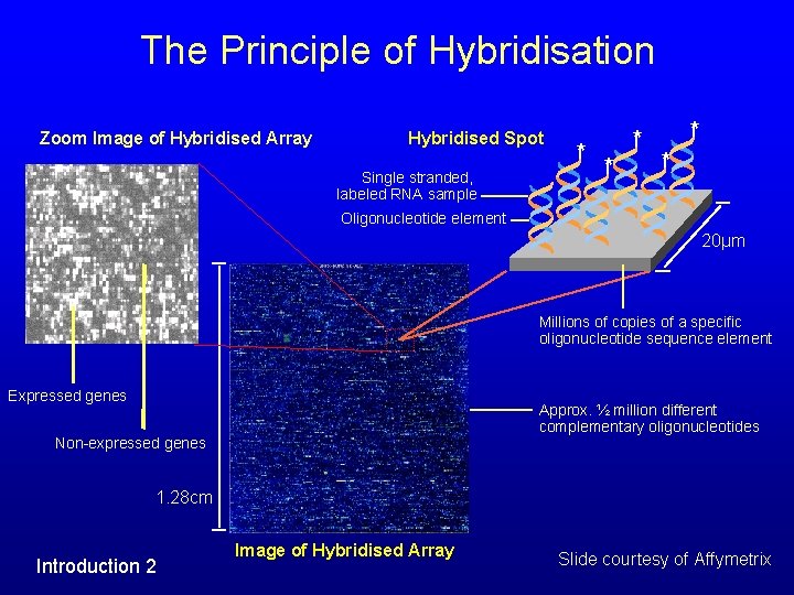
The Principle of Hybridisation Zoom Image of Hybridised Array Hybridised Spot Single stranded, labeled RNA sample * * * Oligonucleotide element 20µm Millions of copies of a specific oligonucleotide sequence element Expressed genes Approx. ½ million different complementary oligonucleotides Non-expressed genes 1. 28 cm Introduction 2 Image of Hybridised Array Slide courtesy of Affymetrix

Hybridisation indicates that the corresponding gene is present because : Ø The binding is highly specific Ø The sequences represented on the array are designed to be unique in the genome The expression level of thousands of genes are measured on a single microarray gene expression profile There are different types of arrays : we consider the case of oligonucleotide arrays where one extract per slide is hybridised Introduction 3

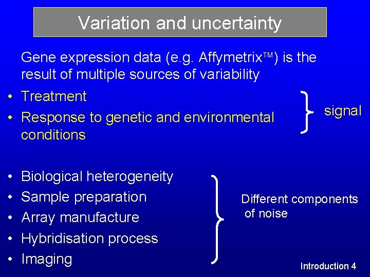
Variation and uncertainty Gene expression data (e. g. Affymetrix ) is the result of multiple sources of variability • Treatment • Response to genetic and environmental conditions • • • Biological heterogeneity Sample preparation Array manufacture Hybridisation process Imaging signal Different components of noise Introduction 4

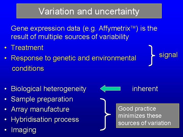
Variation and uncertainty Gene expression data (e. g. Affymetrix ) is the result of multiple sources of variability • Treatment • Response to genetic and environmental conditions • • • Biological heterogeneity Sample preparation Array manufacture Hybridisation process Imaging signal inherent Good practice minimizes these sources of variation

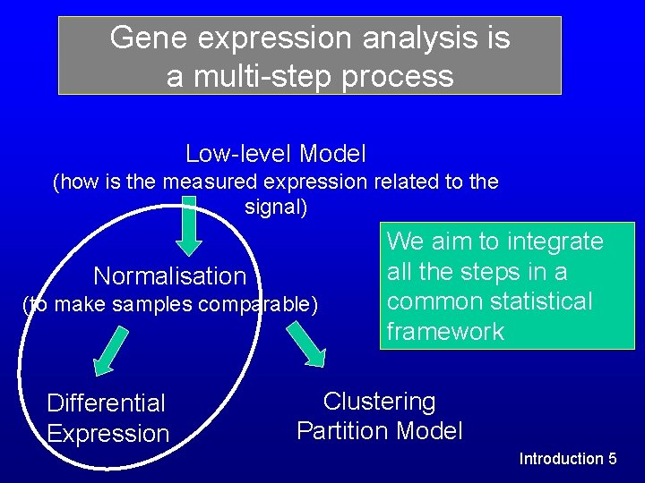
Gene expression analysis is a multi-step process Low-level Model (how is the measured expression related to the signal) Normalisation (to make samples comparable) Differential Expression We aim to integrate all the steps in a common statistical framework Clustering Partition Model Introduction 5

Bayesian hierarchical model framework Ability to model various sources of variability: e. g. detailed modelling of experimental variability: within array, between array, estimation of gene specific variability … Building of all these features into a common model uncertainty is propagated Ability to borrow / share information in appropriate ways to get better estimates Introduction 6

Data Set and Biological question Previous Work (Tim Aitman, Anne Marie Glazier) Deficiency in gene Cd 36 found to be associated with insulin resistance in SHR (spontaneously hypertensive rat) Good animal model to tease out genes implicated in this syndrome Microarray Study • 3 SHR compared with 3 transgenic rats • 3 wildtype mice compared with 3 knockout mice • Two tissues: fat and heart • Affymetrix chips U 34 A-C and U 74 A-C ( 12000 genes)

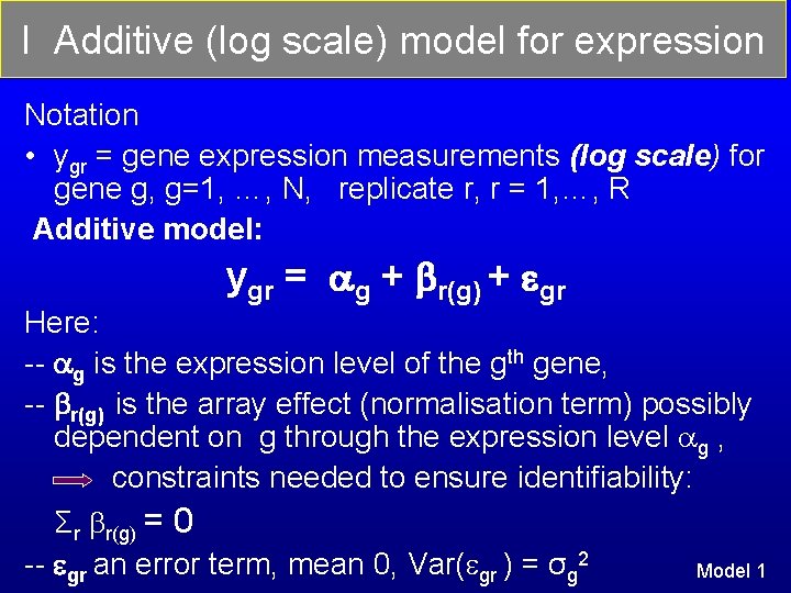
I Additive (log scale) model for expression Notation • ygr = gene expression measurements (log scale) for gene g, g=1, …, N, replicate r, r = 1, …, R Additive model: ygr = g + r(g) + gr Here: -- g is the expression level of the gth gene, -- r(g) is the array effect (normalisation term) possibly dependent on g through the expression level g , constraints needed to ensure identifiability: Σr r(g) = 0 -- gr an error term, mean 0, Var( gr ) = σg 2 Model 1

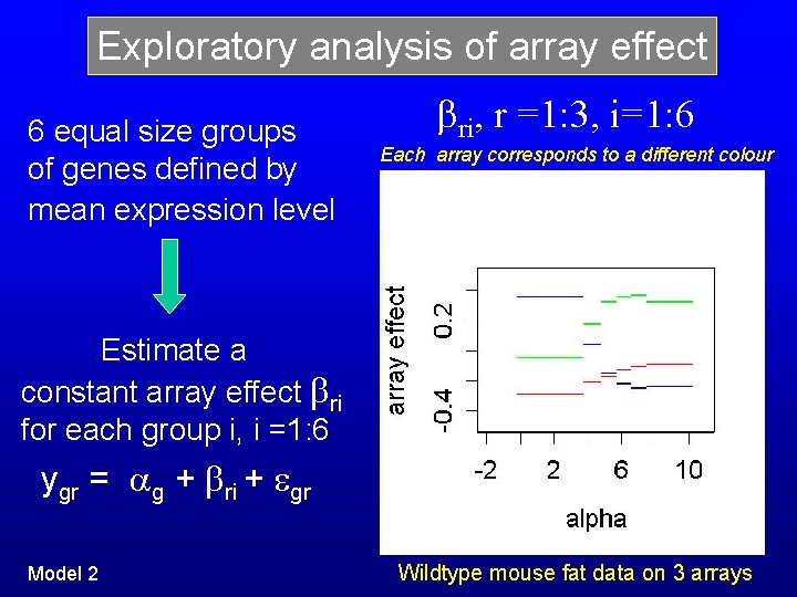
Exploratory analysis of array effect 6 equal size groups of genes defined by mean expression level ri, r =1: 3, i=1: 6 Each array corresponds to a different colour Estimate a constant array effect ri for each group i, i =1: 6 ygr = g + ri + gr Model 2 Wildtype mouse fat data on 3 arrays

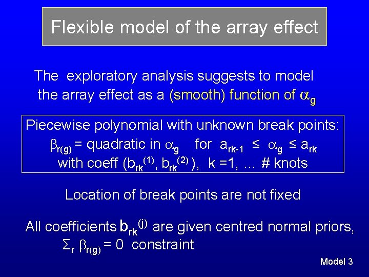
Flexible model of the array effect The exploratory analysis suggests to model the array effect as a (smooth) function of g Piecewise polynomial with unknown break points: r(g) = quadratic in g for ark-1 ≤ g ≤ ark with coeff (brk(1), brk(2) ), k =1, … # knots Location of break points are not fixed All coefficients brk(j) are given centred normal priors, Σr r(g) = 0 constraint Model 3

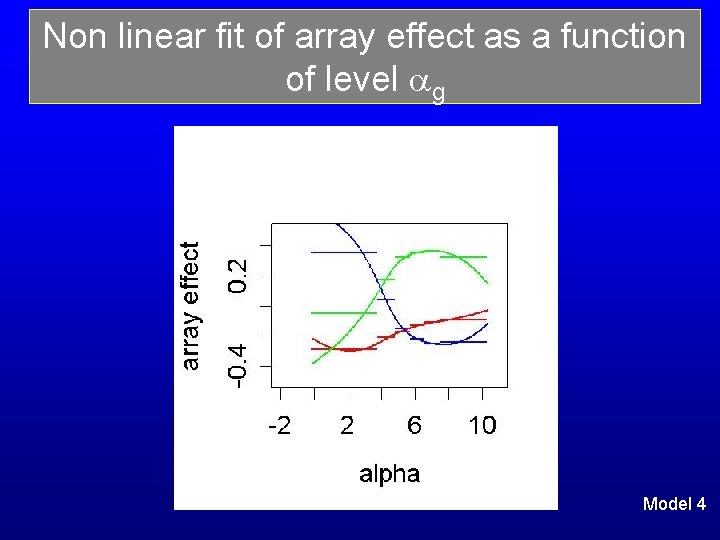
Non linear fit of array effect as a function of level g Model 4

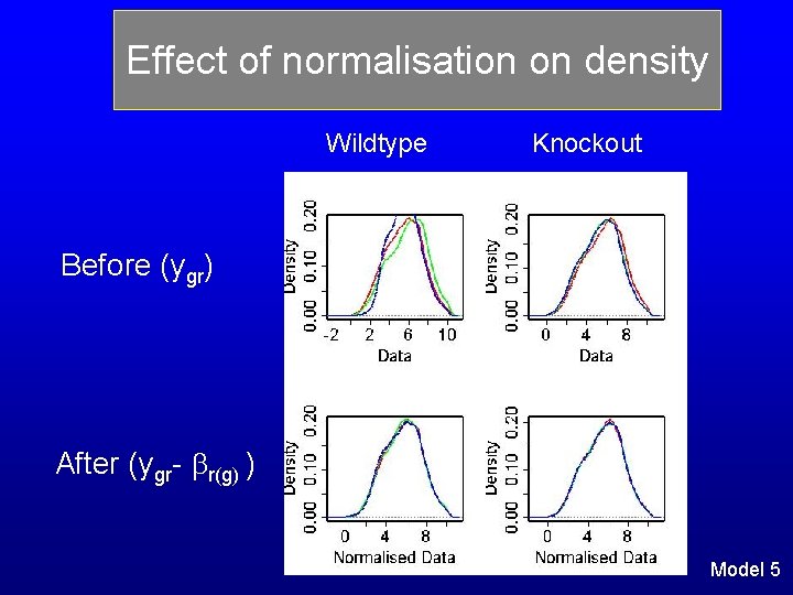
Effect of normalisation on density Wildtype Knockout Before (ygr) After (ygr- r(g) ) Model 5

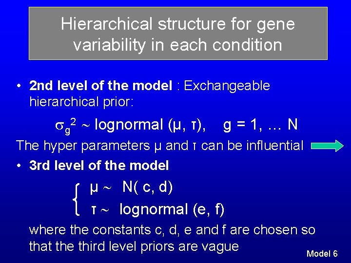
Hierarchical structure for gene variability in each condition • 2 nd level of the model : Exchangeable hierarchical prior: g 2 lognormal (μ, τ), g = 1, … N The hyper parameters μ and τ can be influential • 3 rd level of the model μ N( c, d) τ lognormal (e, f) where the constants c, d, e and f are chosen so that the third level priors are vague Model 6

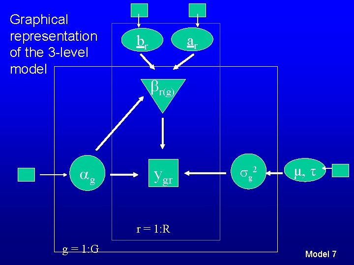
Graphical representation of the 3 -level model g ar br r(g) ygr g 2 μ, τ r = 1: R g = 1: G Model 7

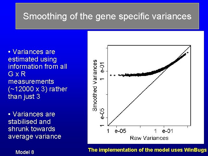
Smoothing of the gene specific variances • Variances are estimated using information from all Gx. R measurements (~12000 x 3) rather than just 3 • Variances are stabilised and shrunk towards average variance Model 8 The implementation of the model uses Win. Bugs

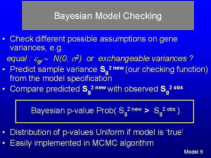
Bayesian Model Checking • Check different possible assumptions on gene variances, e. g. equal : gr N(0, 2) or exchangeable variances ? • Predict sample variance Sg 2 new (our checking function) from the model specification • Compare predicted Sg 2 new with observed Sg 2 obs Bayesian p-value Prob( Sg 2 new > Sg 2 obs ) • Distribution of p-values Uniform if model is ‘true’ • Easily implemented in MCMC algorithm Model 9

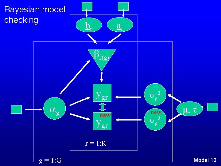
Bayesian model checking ar br r(g) ygr g new ygr g 2 new g 2 μ, τ r = 1: R g = 1: G Model 10

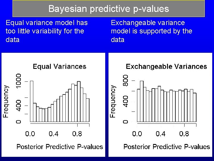
Bayesian predictive p-values Equal variance model has too little variability for the data Exchangeable variance model is supported by the data

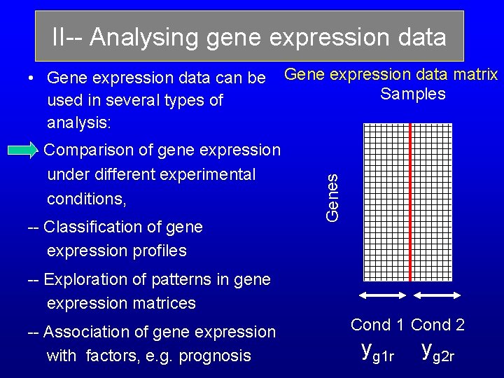
II-- Analysing gene expression data -- Comparison of gene expression under different experimental conditions, -- Classification of gene expression profiles Gene expression data matrix Samples Genes • Gene expression data can be used in several types of analysis: -- Exploration of patterns in gene expression matrices -- Association of gene expression with factors, e. g. prognosis Cond 1 Cond 2 yg 1 r yg 2 r

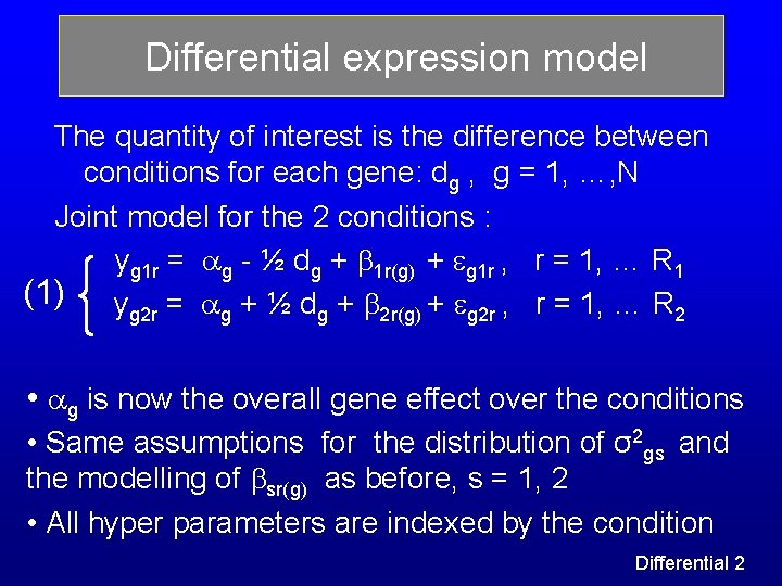
Differential expression model The quantity of interest is the difference between conditions for each gene: dg , g = 1, …, N Joint model for the 2 conditions : yg 1 r = g - ½ dg + 1 r(g) + g 1 r , r = 1, … R 1 (1) y = + ½ d + + , r = 1, … R g 2 r g g 2 r(g) g 2 r 2 • g is now the overall gene effect over the conditions • Same assumptions for the distribution of σ2 gs and the modelling of sr(g) as before, s = 1, 2 • All hyper parameters are indexed by the condition Differential 2

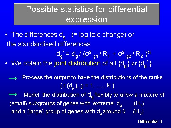
Possible statistics for differential expression • The differences dg (≈ log fold change) or the standardised differences dg* = dg / (σ2 g 1 / R 1 + σ2 g 2 / R 2 )½ • We obtain the joint distribution of all {dg } or {dg* } Process the output to have the distributions of the ranks { r (dg ), g = 1, …. , N } Model the distribution of dg flexibly to allow a mixture of (small) subgroups of genes with ‘extreme’ dg (H 1) and a (large) group of genes with dg around 0 (H 0) Differential 3

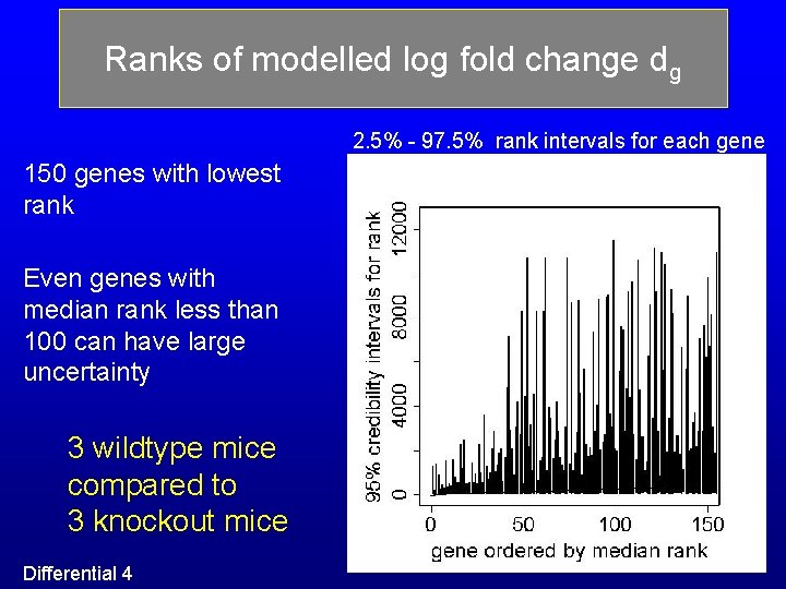
Ranks of modelled log fold change dg 2. 5% - 97. 5% rank intervals for each gene 150 genes with lowest rank Even genes with median rank less than 100 can have large uncertainty 3 wildtype mice compared to 3 knockout mice Differential 4

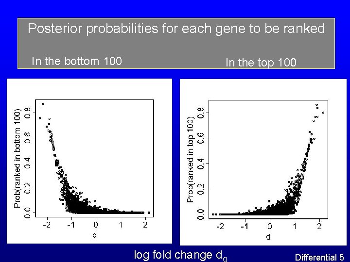
Posterior probabilities for each gene to be ranked In the bottom 100 In the top 100 log fold change dg Differential 5

Mixture modelling the distribution of dg • Mixture model framework but with an ‘unknown’ number of components • Fully Bayesian hierarchical framework (the number of components is a random variable) • Based on Green (1995) and Richardson and Green (1997) papers • MCMC algorithms • Applied in an experimental context concerning bladder cancer (Broët, Richardson and Radvanyi; Journal of Computational Biology, 9, 671 -683, 2002) Mixture 1

Bayesian mixture model Normal mixtures with an unknown number of states A gene can be in different states: down regulated, …, unaffected, …, up-regulated the central state corresponding to dg ≈ 0 Bayesian estimation of posterior distribution: • for number of states (besides the unaffected one) • for the allocation of genes to the states classification of states in the ‘extreme components’ or in the central one, based on their posterior probability Mixture 2

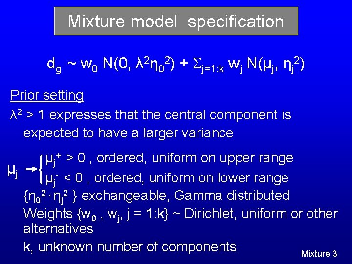
Mixture model specification dg ~ w 0 N(0, λ 2η 02) + j=1: k wj N(μj, ηj 2) Prior setting λ 2 > 1 expresses that the central component is expected to have a larger variance μj+ > 0 , ordered, uniform on upper range μj μj- < 0 , ordered, uniform on lower range {η 02 , ηj 2 } exchangeable, Gamma distributed Weights {w 0 , wj, j = 1: k} ~ Dirichlet, uniform or other alternatives k, unknown number of components Mixture 3

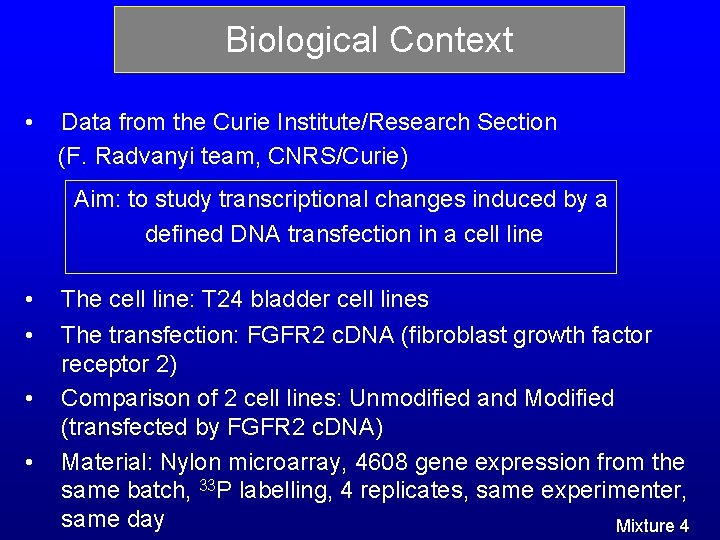
Biological Context • Data from the Curie Institute/Research Section (F. Radvanyi team, CNRS/Curie) Aim: to study transcriptional changes induced by a defined DNA transfection in a cell line • • The cell line: T 24 bladder cell lines The transfection: FGFR 2 c. DNA (fibroblast growth factor receptor 2) Comparison of 2 cell lines: Unmodified and Modified (transfected by FGFR 2 c. DNA) Material: Nylon microarray, 4608 gene expression from the same batch, 33 P labelling, 4 replicates, same experimenter, same day Mixture 4

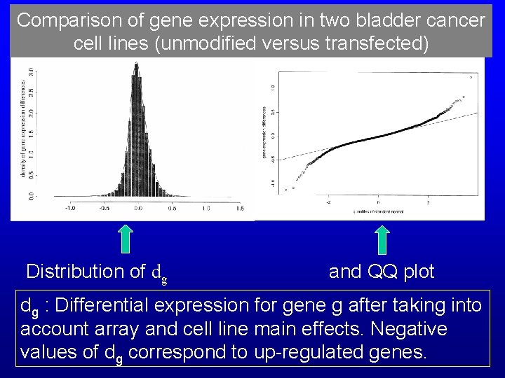
Comparison of gene expression in two bladder cancer cell lines (unmodified versus transfected) Distribution of dg and QQ plot dg : Differential expression for gene g after taking into account array and cell line main effects. Negative values of dg correspond to up-regulated genes.

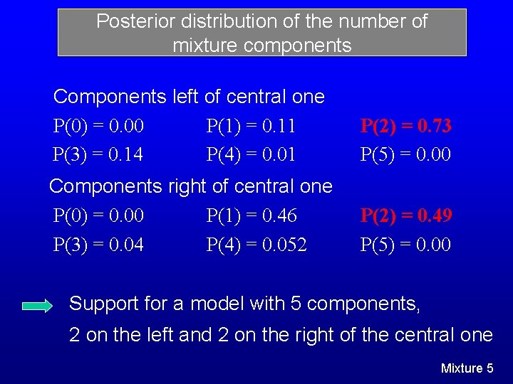
Posterior distribution of the number of mixture components Components left of central one P(0) = 0. 00 P(1) = 0. 11 P(3) = 0. 14 P(4) = 0. 01 P(2) = 0. 73 P(5) = 0. 00 Components right of central one P(0) = 0. 00 P(1) = 0. 46 P(3) = 0. 04 P(4) = 0. 052 P(2) = 0. 49 P(5) = 0. 00 Support for a model with 5 components, 2 on the left and 2 on the right of the central one Mixture 5

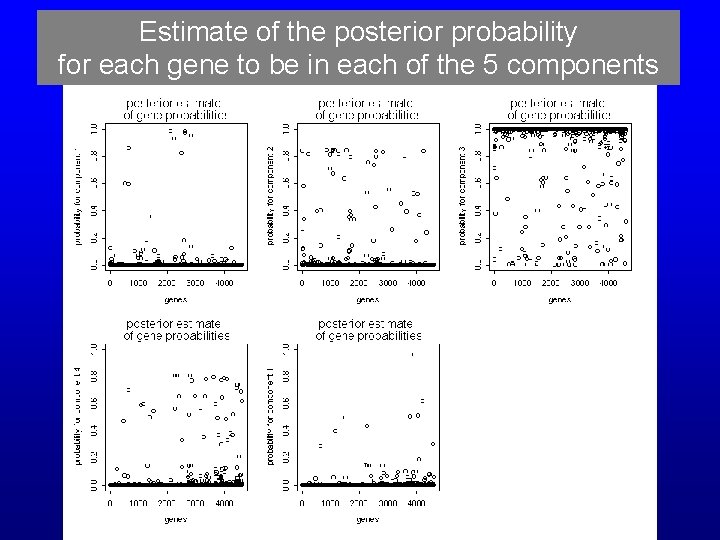
Estimate of the posterior probability for each gene to be in each of the 5 components

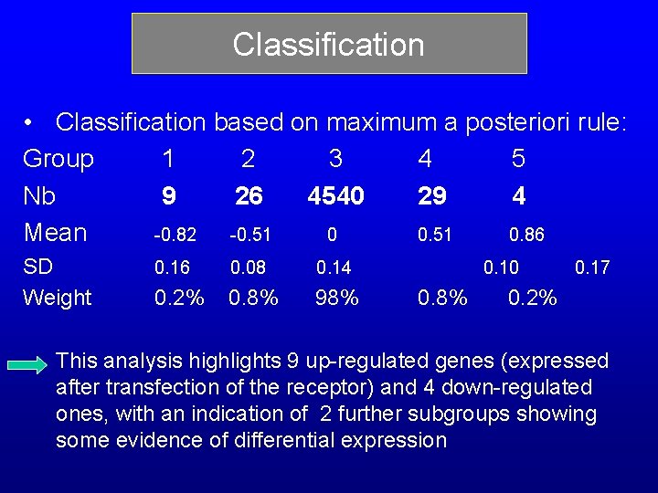
Classification • Classification based on maximum a posteriori rule: Group 1 2 3 4 5 Nb 9 26 4540 29 4 Mean -0. 82 -0. 51 0. 86 SD Weight 0. 16 0. 08 0. 14 0. 2% 0. 8% 98% 0. 10 0. 8% 0. 17 0. 2% This analysis highlights 9 up-regulated genes (expressed after transfection of the receptor) and 4 down-regulated ones, with an indication of 2 further subgroups showing some evidence of differential expression

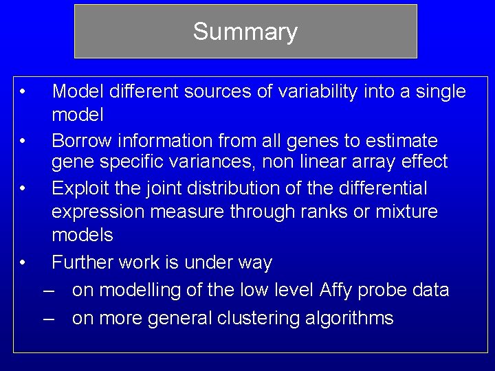
Summary • Model different sources of variability into a single model • Borrow information from all genes to estimate gene specific variances, non linear array effect • Exploit the joint distribution of the differential expression measure through ranks or mixture models • Further work is under way – on modelling of the low level Affy probe data – on more general clustering algorithms