Bayesian mixture models for analysing gene expression data

Bayesian mixture models for analysing gene expression data Natalia Bochkina In collaboration with Alex Lewin , Sylvia Richardson, BAIR Consortium Imperial College London, UK

Introduction We use a fully Bayesian approach to model data and MCMC for parameter estimation. • Models all parameters simultaneously. • Prior information can be included in the model. • Variances are automatically adjusted to avoid unstable estimates for small number of observations. • Inference is based on the posterior distribution of all parameters. • Use the mean of the posterior distribution as an estimate for all parameters.

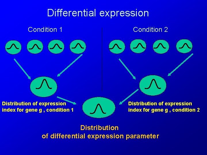
Differential expression Condition 1 Distribution of expression index for gene g , condition 1 Condition 2 Distribution of expression index for gene g , condition 2 Distribution of differential expression parameter

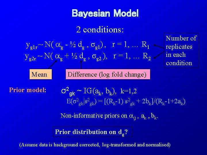
Bayesian Model 2 conditions: yg 1 r ~ N( g - ½ dg , σg 1) , r = 1, … R 1 yg 2 r ~ N( g + ½ dg , σg 2 ), r = 1, … R 2 Mean Prior model: Number of replicates in each condition Difference (log fold change) σ2 gk ~ IG(ak, bk), k=1, 2 E(σ2 gk|s 2 gk) = [(Rk-1) s 2 gk + 2 bk]/(Rk-1+2 ak) Non-informative priors on g , ak , bk. Prior distribution on dg? (Assume data is background corrected, log-transformed and normalised)

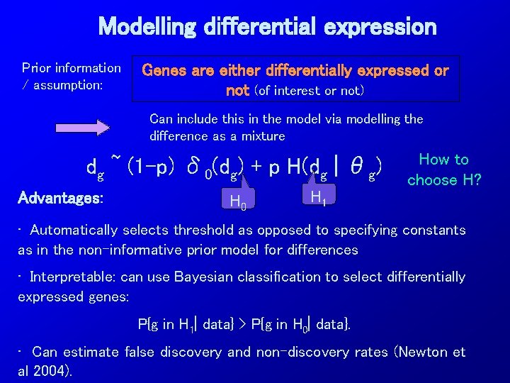
Modelling differential expression Prior information / assumption: Genes are either differentially expressed or not (of interest or not) Can include this in the model via modelling the difference as a mixture dg ~ (1 -p) δ 0(dg) + p H(dg | θg) Advantages: H 0 H 1 How to choose H? • Automatically selects threshold as opposed to specifying constants as in the non-informative prior model for differences • Interpretable: can use Bayesian classification to select differentially expressed genes: P{g in H 1| data} > P{g in H 0| data}. • Can estimate false discovery and non-discovery rates (Newton et al 2004).

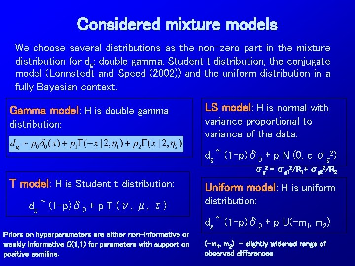
Considered mixture models We choose several distributions as the non-zero part in the mixture distribution for dg: double gamma, Student t distribution, the conjugate model (Lonnstedt and Speed (2002)) and the uniform distribution in a fully Bayesian context. Gamma model: H is double gamma distribution: LS model: H is normal with variance proportional to variance of the data: dg ~ (1 -p)δ 0 + p N (0, c σg 2) σg 2 = σg 12/R 1+ σg 22/R 2 T model: H is Student t distribution: dg ~ (1 -p)δ 0 + p T (ν, μ, τ) Uniform model: H is uniform distribution: dg ~ (1 -p)δ 0 + p U(-m 1, m 2) Priors on hyperparameters are either non-informative or weakly informative G(1, 1) for parameters with support on positive semiline. (-m 1, m 2) - slightly widened range of observed differences

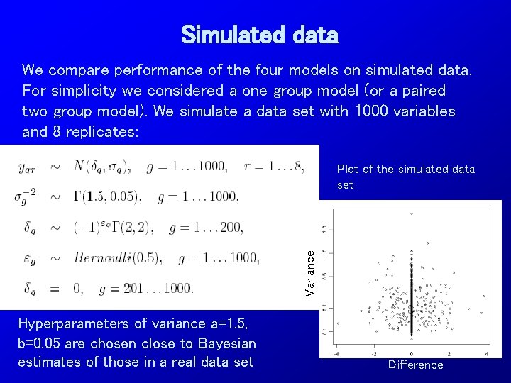
Simulated data We compare performance of the four models on simulated data. For simplicity we considered a one group model (or a paired two group model). We simulate a data set with 1000 variables and 8 replicates: Variance Plot of the simulated data set Hyperparameters of variance a=1. 5, b=0. 05 are chosen close to Bayesian estimates of those in a real data set Difference

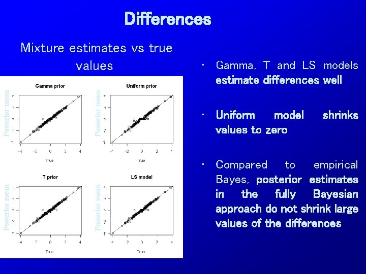
Differences Posterior mean • Gamma, T and LS models estimate differences well • Uniform model values to zero Posterior mean Mixture estimates vs true values • Compared to empirical Bayes, posterior estimates in the fully Bayesian approach do not shrink large values of the differences shrinks

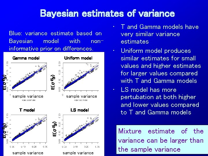
Bayesian estimates of variance Blue: variance estimate based on Bayesian model with noninformative prior on differences. Uniform model E(σ2|y) Gamma model sample variance LS model E(σ2|y) T model sample variance • T and Gamma models have very similar variance estimates • Uniform model produces similar estimates for small values and higher estimates for larger values compared with T and Gamma models • LS model has more pertubation at both higher and lower values compared to T and Gamma models Mixture estimate of the variance can be larger than the sample variance

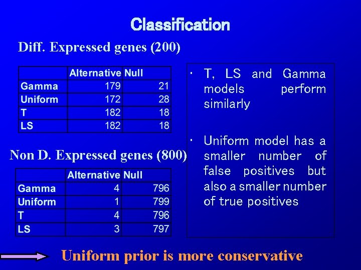
Classification Diff. Expressed genes (200) • T, LS and Gamma models perform similarly • Uniform model has a Non D. Expressed genes (800) smaller number of false positives but also a smaller number of true positives Uniform prior is more conservative

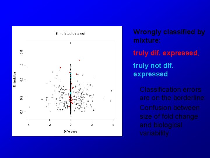
Wrongly classified by mixture: truly dif. expressed, truly not dif. expressed Classification errors are on the borderline: Confusion between size of fold change and biological variability

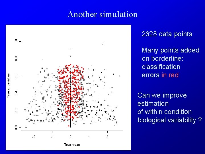
Another simulation 2628 data points Many points added on borderline: classification errors in red Can we improve estimation of within condition biological variability ?

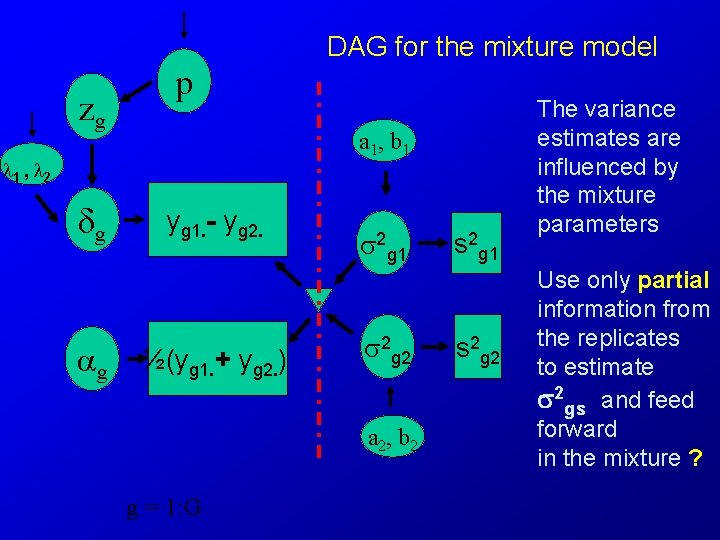
DAG for the mixture model zg p a 1, b 1 1 , 2 δg g yg 1. - yg 2. ½(yg 1. + yg 2. ) 2 g 1 2 g 2 a 2, b 2 g = 1: G s 2 g 1 s 2 g 2 The variance estimates are influenced by the mixture parameters Use only partial information from the replicates to estimate 2 gs and feed forward in the mixture ?

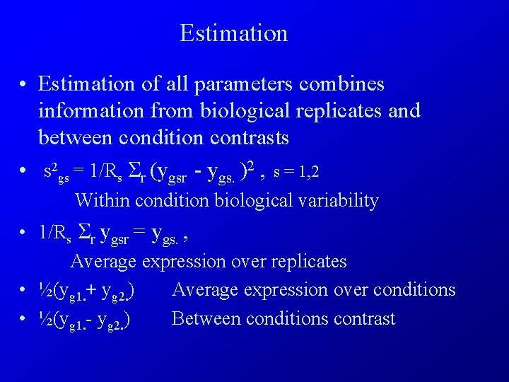
Estimation • Estimation of all parameters combines information from biological replicates and between condition contrasts • s 2 gs = 1/Rs Σr (ygsr - ygs. )2 , s = 1, 2 Within condition biological variability • 1/Rs Σr ygsr = ygs. , Average expression over replicates • ½(yg 1. + yg 2. ) Average expression over conditions • ½(yg 1. - yg 2. ) Between conditions contrast

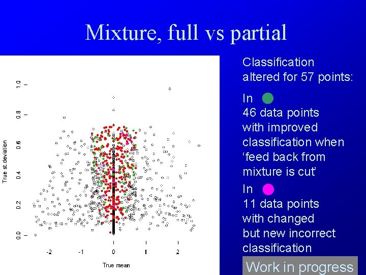
Mixture, full vs partial Classification altered for 57 points: In 46 data points with improved classification when ‘feed back from mixture is cut’ In 11 data points with changed but new incorrect classification Work in progress

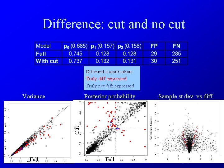
Difference: cut and no cut Different classification: Truly diff. expressed Truly not diff. expressed Posterior probability Cut Variance Full Sample st. dev. vs diff.

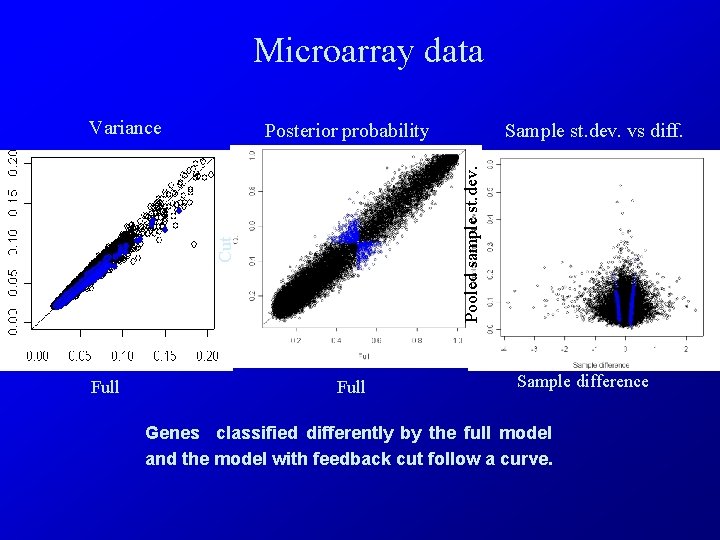
Microarray data Variance Cut Full Sample st. dev. vs diff. Pooled sample st. dev. Posterior probability Full Sample difference Genes classified differently by the full model and the model with feedback cut follow a curve.

Since variance is overestimated in full mixture model compared to mixture model with cut, the number of False Negatives is lower for model with cut than for the full model.

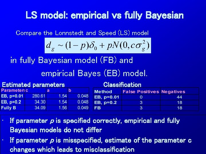
LS model: empirical vs fully Bayesian Compare the Lonnstedt and Speed (LS) model in fully Bayesian model (FB) and empirical Bayes (EB) model. Estimated parameters Classification • If parameter p is specified correctly, empirical and fully Bayesian models do not differ • If parameter p is misspecified, estimate of the parameter c changes which leads to misclassification

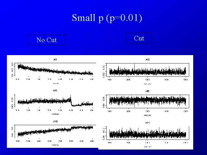
Small p (p=0. 01) No Cut

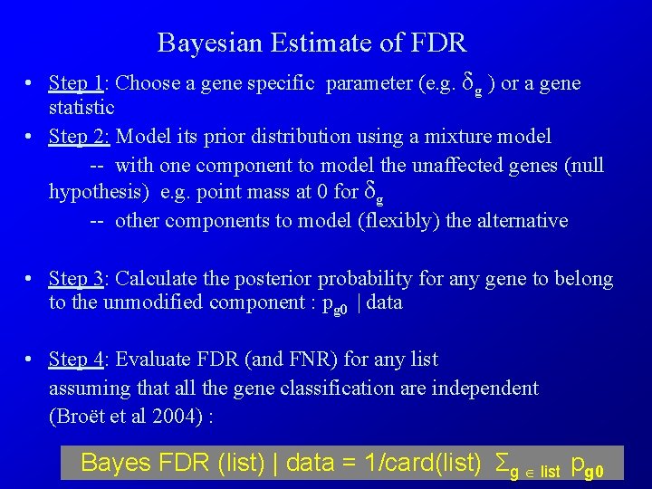
Bayesian Estimate of FDR • Step 1: Choose a gene specific parameter (e. g. δg ) or a gene statistic • Step 2: Model its prior distribution using a mixture model -- with one component to model the unaffected genes (null hypothesis) e. g. point mass at 0 for δg -- other components to model (flexibly) the alternative • Step 3: Calculate the posterior probability for any gene to belong to the unmodified component : pg 0 | data • Step 4: Evaluate FDR (and FNR) for any list assuming that all the gene classification are independent (Broët et al 2004) : Bayes FDR (list) | data = 1/card(list) Σg list pg 0

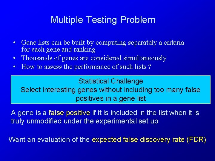
Multiple Testing Problem • Gene lists can be built by computing separately a criteria for each gene and ranking • Thousands of genes are considered simultaneously • How to assess the performance of such lists ? Statistical Challenge Select interesting genes without including too many false positives in a gene list A gene is a false positive if it is included in the list when it is truly unmodified under the experimental set up Want an evaluation of the expected false discovery rate (FDR)

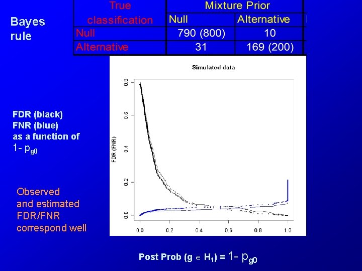
Bayes rule FDR (black) FNR (blue) as a function of 1 - pg 0 Observed and estimated FDR/FNR correspond well Post Prob (g H 1) = 1 - pg 0

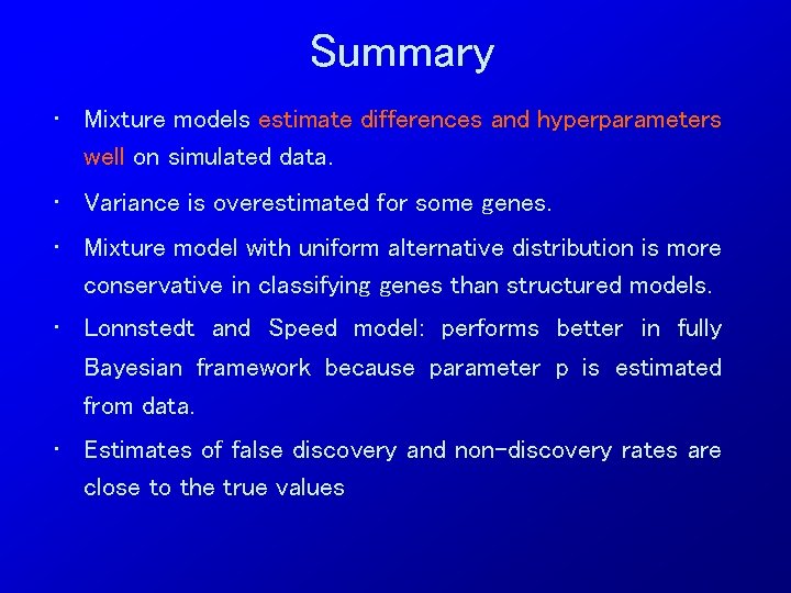
Summary • Mixture models estimate differences and hyperparameters well on simulated data. • Variance is overestimated for some genes. • Mixture model with uniform alternative distribution is more conservative in classifying genes than structured models. • Lonnstedt and Speed model: performs better in fully Bayesian framework because parameter p is estimated from data. • Estimates of false discovery and non-discovery rates are close to the true values