Bayesian Linear Regression Introducing GLM Important Variable Descriptors

Bayesian Linear Regression

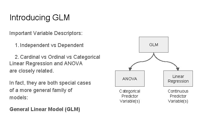
Introducing GLM Important Variable Descriptors: 1. Independent vs Dependent GLM 2. Cardinal vs Ordinal vs Categorical Linear Regression and ANOVA are closely related. In fact, they are both special cases of a more general family of models: General Linear Model (GLM) ANOVA Linear Regression Categorical Predictor Variable(s) Continuous Predictor Variable(s)

OLS Linear Regression Worked Example

Against Causality If a dependent variable depends on an independent variable, that still doesn’t conclusively demonstrate causality nor temporal priority. Height can depend on weight, but doesn’t “happen first” Similarly, even if a linear regression model provides a lot of predictive power, Y might still be causally disconnected from X.

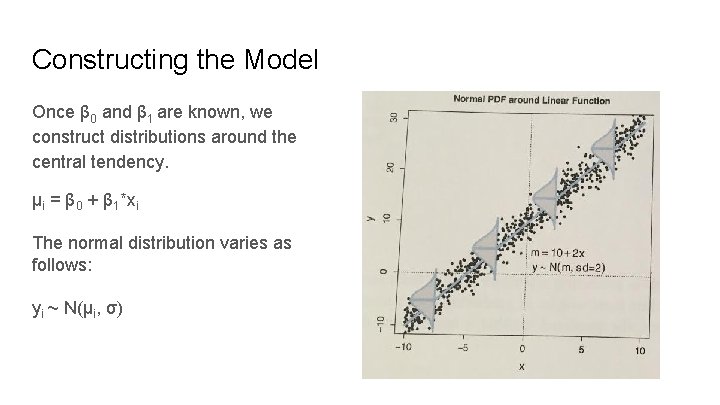
Constructing the Model Once β 0 and β 1 are known, we construct distributions around the central tendency. μi = β 0 + β 1*xi The normal distribution varies as follows: yi ~ N(μi, σ)

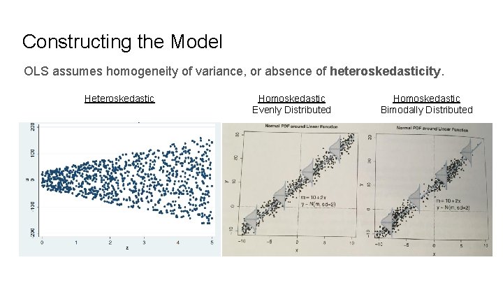
Constructing the Model OLS assumes homogeneity of variance, or absence of heteroskedasticity. Heteroskedastic Homoskedastic Evenly Distributed Homoskedastic Bimodally Distributed

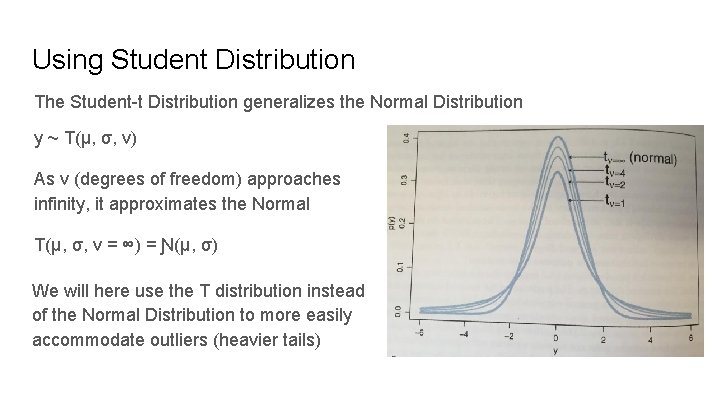
Using Student Distribution The Student-t Distribution generalizes the Normal Distribution y ~ T(μ, σ, v) As v (degrees of freedom) approaches infinity, it approximates the Normal T(μ, σ, v = ∞) = Ɲ(μ, σ) We will here use the T distribution instead of the Normal Distribution to more easily accommodate outliers (heavier tails)

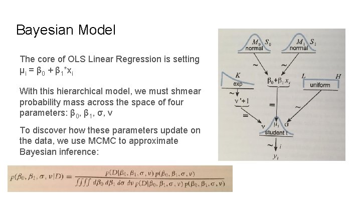
Bayesian Model The core of OLS Linear Regression is setting μi = β 0 + β 1*xi With this hierarchical model, we must shmear probability mass across the space of four parameters: β 0, β 1, σ, v To discover how these parameters update on the data, we use MCMC to approximate Bayesian inference:

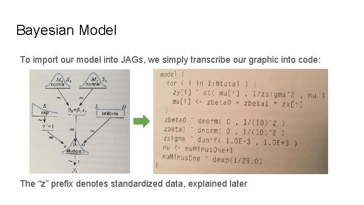
Bayesian Model To import our model into JAGs, we simply transcribe our graphic into code: The “z” prefix denotes standardized data, explained later

Data Normalization In frequentist OLS, it is considered best practice to mean-center your IVs: X’ = X - μx For Bayesian Inference, we will go a bit further & standardize: X’ = (X - μx) / σx What’s the point? Mean Centering: Decorrelates parameters Normalization: priors less sensitive to scale of the data

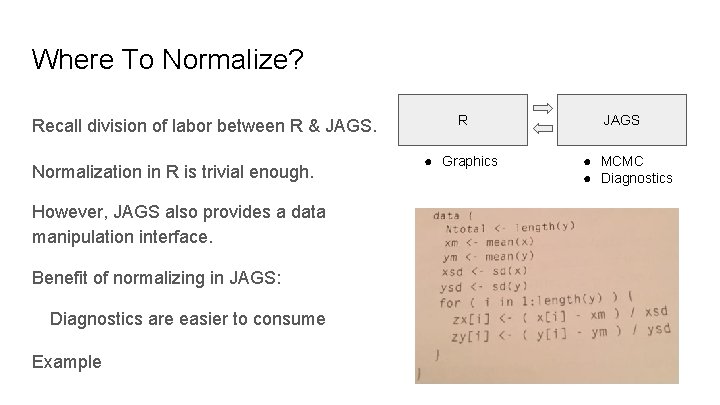
Where To Normalize? Recall division of labor between R & JAGS. Normalization in R is trivial enough. However, JAGS also provides a data manipulation interface. Benefit of normalizing in JAGS: Diagnostics are easier to consume Example R ● Graphics JAGS ● MCMC ● Diagnostics

Bayesian Linear Regression JAGS Implementation