Bayesian Interval Mapping 1 what is Bayes Bayes

Bayesian Interval Mapping 1. what is Bayes? Bayes theorem? 2 -6 2. Bayesian QTL mapping 7 -17 3. Markov chain sampling 18 -25 4. sampling across architectures 26 -32 Bayes NCSU QTL II: Yandell © 2005 1

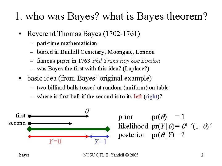
1. who was Bayes? what is Bayes theorem? • Reverend Thomas Bayes (1702 -1761) – – part-time mathematician buried in Bunhill Cemetary, Moongate, London famous paper in 1763 Phil Trans Roy Soc London was Bayes the first with this idea? (Laplace? ) • basic idea (from Bayes’ original example) – two billiard balls tossed at random (uniform) on table – where is first ball if the second is to its left (right)? first second Y=0 Bayes Y=1 prior pr( ) = 1 likelihood pr(Y | )= 1–Y(1– )Y posterior pr( |Y) = ? NCSU QTL II: Yandell © 2005 2

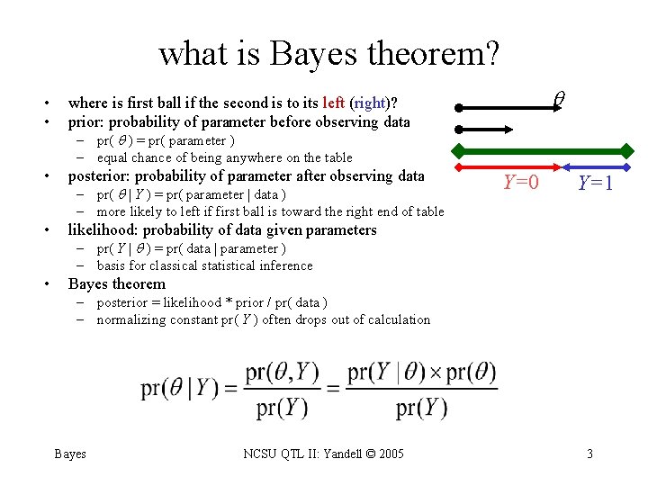
what is Bayes theorem? • • where is first ball if the second is to its left (right)? prior: probability of parameter before observing data • posterior: probability of parameter after observing data • likelihood: probability of data given parameters • Bayes theorem – pr( ) = pr( parameter ) – equal chance of being anywhere on the table – pr( | Y ) = pr( parameter | data ) – more likely to left if first ball is toward the right end of table Y=0 Y=1 – pr( Y | ) = pr( data | parameter ) – basis for classical statistical inference – posterior = likelihood * prior / pr( data ) – normalizing constant pr( Y ) often drops out of calculation Bayes NCSU QTL II: Yandell © 2005 3

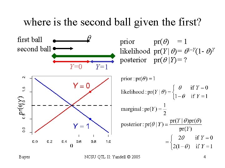
where is the second ball given the first? first ball second ball Y=0 Bayes

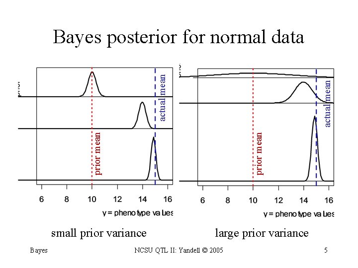
prior mean actual mean Bayes posterior for normal data small prior variance Bayes large

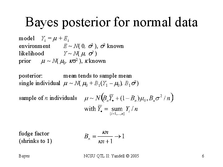
Bayes posterior for normal data model Yi = + Ei environment E ~ N( 0, 2 ), 2 known likelihood Y ~ N( , 2 ) prior ~ N( 0, 2 ), known posterior: mean tends to sample mean single individual ~ N( 0 + B 1(Y 1 – 0), B 1 2) sample of n individuals fudge factor (shrinks to 1) Bayes NCSU QTL II: Yandell © 2005 6

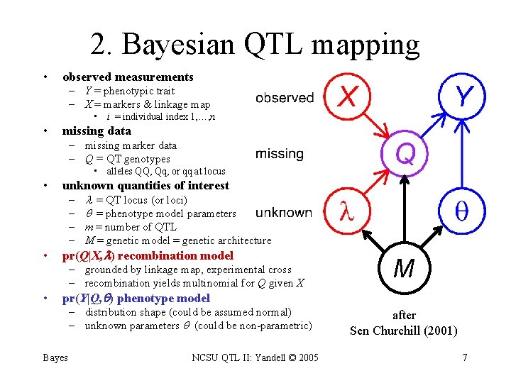
2. Bayesian QTL mapping • observed measurements – Y = phenotypic trait – X = markers & linkage map • i = individual index 1, …, n • missing data – missing marker data – Q = QT genotypes • alleles QQ, Qq, or qq at locus • unknown quantities of interest – – • = QT locus (or loci) = phenotype model parameters m = number of QTL M = genetic model = genetic architecture pr(Q|X, ) recombination model – grounded by linkage map, experimental cross – recombination yields multinomial for Q given X • M pr(Y|Q, ) phenotype model – distribution shape (could be assumed normal) – unknown parameters (could be non-parametric) Bayes NCSU QTL II: Yandell © 2005 after Sen Churchill (2001) 7

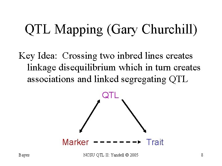
QTL Mapping (Gary Churchill) Key Idea: Crossing two inbred lines creates linkage disequilibrium which in turn creates associations and linked segregating QTL Marker Bayes NCSU QTL II: Yandell © 2005 Trait 8

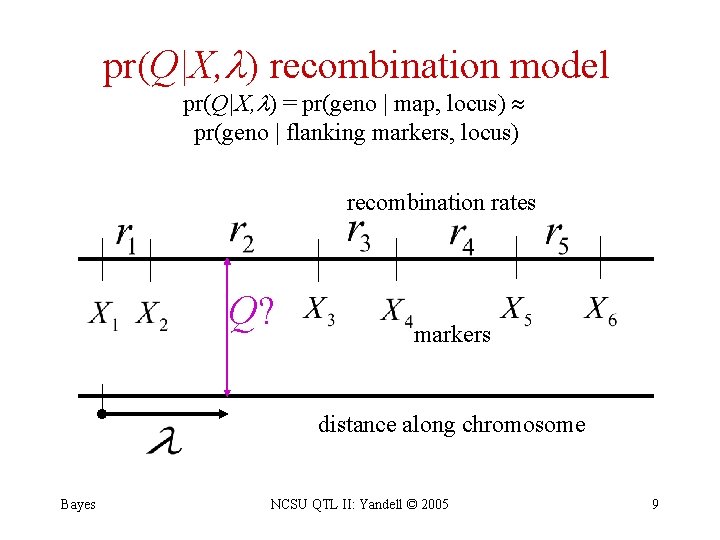
pr(Q|X, ) recombination model pr(Q|X, ) = pr(geno | map, locus) pr(geno | flanking

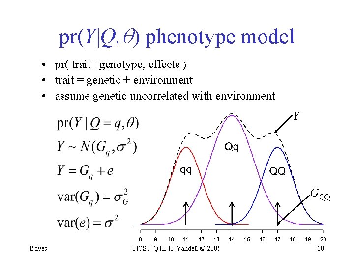
pr(Y|Q, ) phenotype model • pr( trait | genotype, effects ) • trait =

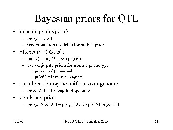
Bayesian priors for QTL • missing genotypes Q – pr( Q | X, ) – recombination model is formally a prior • effects = ( G, 2 ) – pr( ) = pr( Gq | 2 ) pr( 2 ) – use conjugate priors for normal phenotype • pr( Gq | 2 ) = normal • pr( 2 ) = inverse chi-square • each locus may be uniform over genome – pr( | X ) = 1 / length of genome • combined prior – pr( Q, , | X ) = pr( Q | X, ) pr( | X ) Bayes NCSU QTL II: Yandell © 2005 11

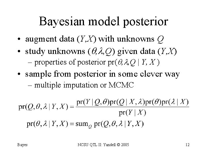
Bayesian model posterior • augment data (Y, X) with unknowns Q • study unknowns ( , , Q) given data (Y, X) – properties of posterior pr( , , Q | Y, X ) • sample from posterior in some clever way – multiple imputation or MCMC Bayes NCSU QTL II: Yandell © 2005 12

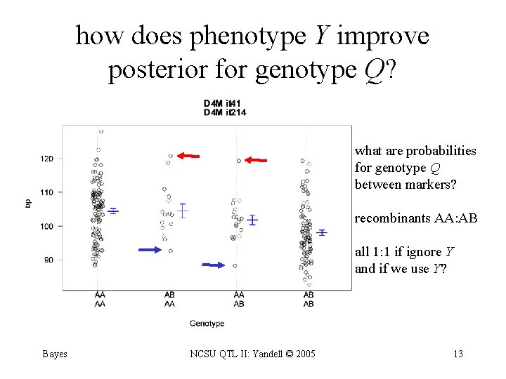
how does phenotype Y improve posterior for genotype Q? what are probabilities for genotype Q between markers? recombinants AA: AB all 1: 1 if ignore Y and if we use Y? Bayes NCSU QTL II: Yandell © 2005 13

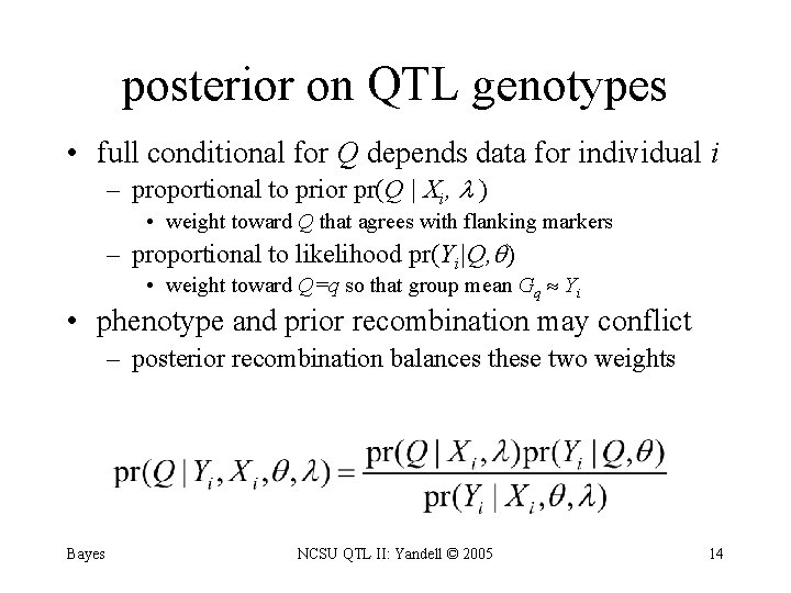
posterior on QTL genotypes • full conditional for Q depends data for individual i – proportional to prior pr(Q | Xi, ) • weight toward Q that agrees with flanking markers – proportional to likelihood pr(Yi|Q, ) • weight toward Q=q so that group mean Gq Yi • phenotype and prior recombination may conflict – posterior recombination balances these two weights Bayes NCSU QTL II: Yandell © 2005 14

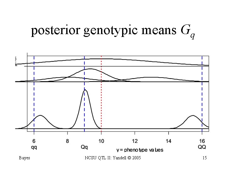
posterior genotypic means Gq Bayes NCSU QTL II: Yandell © 2005 15

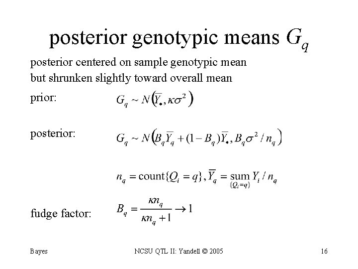
posterior genotypic means Gq posterior centered on sample genotypic mean but shrunken slightly toward

What if variance 2 is unknown? • sample variance is proportional to chi-square – ns 2 / 2 ~ 2 ( n ) – likelihood of sample variance s 2 given n, 2 • conjugate prior is inverse chi-square – 2 / 2 ~ 2 ( ) – prior of population variance 2 given , 2 • posterior is weighted average of likelihood and prior – ( 2+ns 2) / 2 ~ 2 ( +n ) – posterior of population variance 2 given n, s 2, , 2 • empirical choice of hyper-parameters – 2= s 2/3, =6 – E( 2 | , 2) = s 2/2, Var( 2 | , 2) = s 4/4 Bayes NCSU QTL II: Yandell © 2005 17

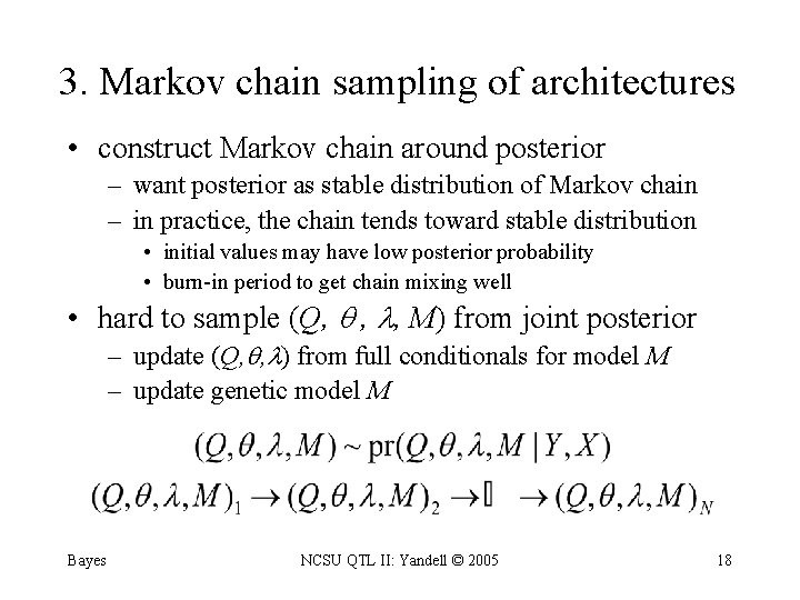
3. Markov chain sampling of architectures • construct Markov chain around posterior – want posterior as stable distribution of Markov chain – in practice, the chain tends toward stable distribution • initial values may have low posterior probability • burn-in period to get chain mixing well • hard to sample (Q, , , M) from joint posterior – update (Q, , ) from full conditionals for model M – update genetic model M Bayes NCSU QTL II: Yandell © 2005 18

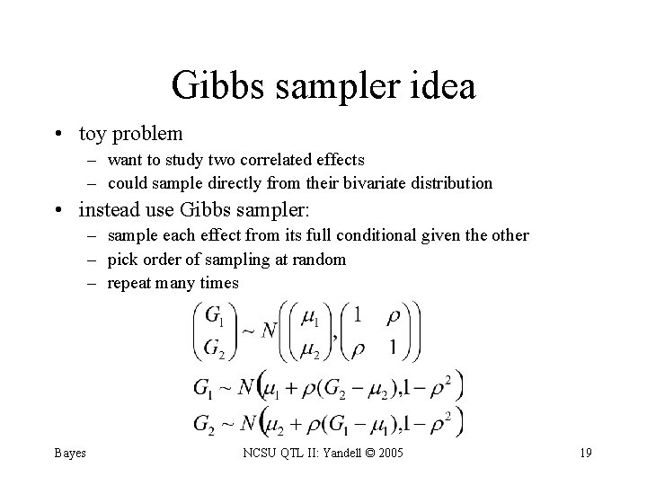
Gibbs sampler idea • toy problem – want to study two correlated effects – could sample directly from their bivariate distribution • instead use Gibbs sampler: – sample each effect from its full conditional given the other – pick order of sampling at random – repeat many times Bayes NCSU QTL II: Yandell © 2005 19

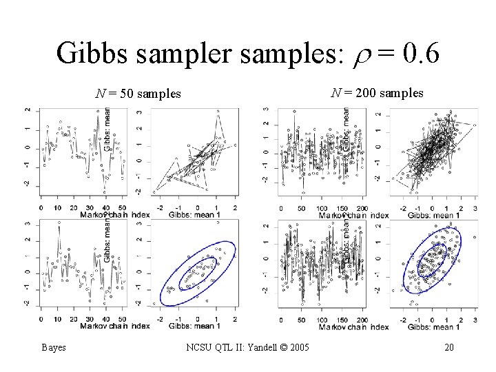
Gibbs sampler samples: = 0. 6 N = 200 samples N = 50 samples

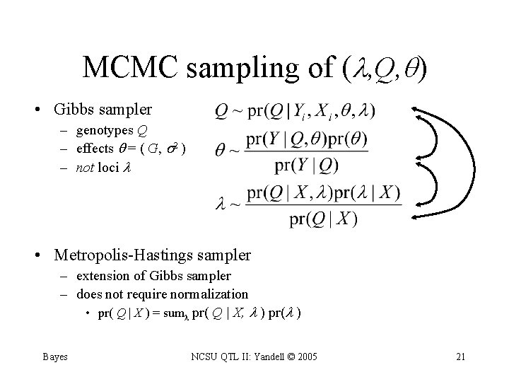
MCMC sampling of ( , Q, ) • Gibbs sampler – genotypes Q – effects = ( G, 2 ) – not loci • Metropolis-Hastings sampler – extension of Gibbs sampler – does not require normalization • pr( Q | X ) = sum pr( Q | X, ) pr( ) Bayes NCSU QTL II: Yandell © 2005 21

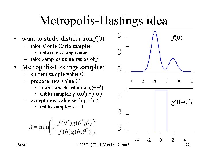
Metropolis-Hastings idea • want to study distribution f( ) – take Monte Carlo samples • unless too complicated – take samples using ratios of f • Metropolis-Hastings samples: – current sample value – propose new value * • from some distribution g( , *) • Gibbs sampler: g( , *) = f( *) – accept new value with prob A • Gibbs sampler: A = 1 Bayes NCSU QTL II: Yandell © 2005 g( – *) 22

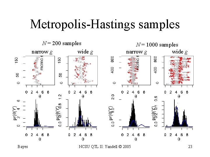
Metropolis-Hastings samples N = 200 samples narrow g wide g Bayes N = 1000

full conditional for locus • cannot easily sample from locus full conditional pr( |Y, X, , Q) = pr( | X, Q) = pr( Q | X, ) pr( ) / constant • constant is very difficult to compute explicitly – must average over all possible loci over genome – must do this for every possible genotype Q • Gibbs sampler will not work in general – but can use method based on ratios of probabilities – Metropolis-Hastings is extension of Gibbs sampler Bayes NCSU QTL II: Yandell © 2005 24

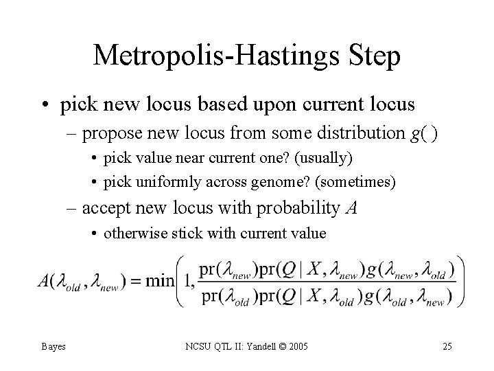
Metropolis-Hastings Step • pick new locus based upon current locus – propose new locus from some distribution g( ) • pick value near current one? (usually) • pick uniformly across genome? (sometimes) – accept new locus with probability A • otherwise stick with current value Bayes NCSU QTL II: Yandell © 2005 25

4. sampling across architectures • search across genetic architectures M of various sizes – allow change in m = number of QTL – allow change in types of epistatic interactions • methods for search – reversible jump MCMC – Gibbs sampler with loci indicators • complexity of epistasis – Fisher-Cockerham effects model – general multi-QTL interaction & limits of inference Bayes NCSU QTL II: Yandell © 2005 26

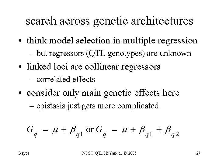
search across genetic architectures • think model selection in multiple regression – but regressors (QTL genotypes) are unknown • linked loci are collinear regressors – correlated effects • consider only main genetic effects here – epistasis just gets more complicated Bayes NCSU QTL II: Yandell © 2005 27

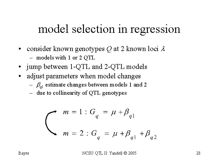
model selection in regression • consider known genotypes Q at 2 known loci – models with 1 or 2 QTL • jump between 1 -QTL and 2 -QTL models • adjust parameters when model changes – q 1 estimate changes between models 1 and 2 – due to collinearity of QTL genotypes Bayes NCSU QTL II: Yandell © 2005 28

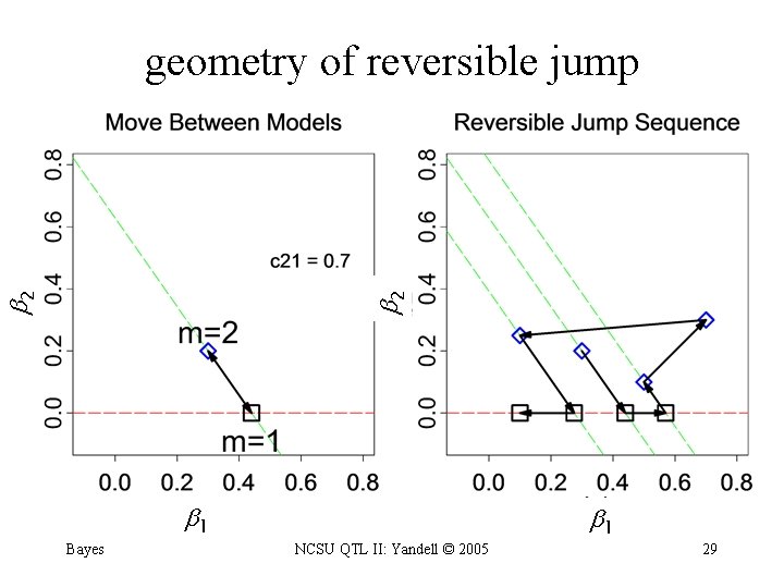
2 2 geometry of reversible jump 1 Bayes NCSU QTL II: Yandell ©

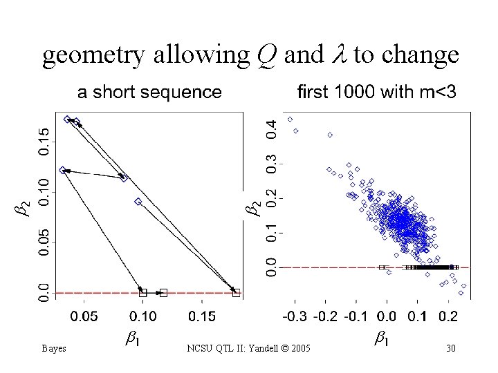
2 2 geometry allowing Q and to change Bayes 1 NCSU QTL II:

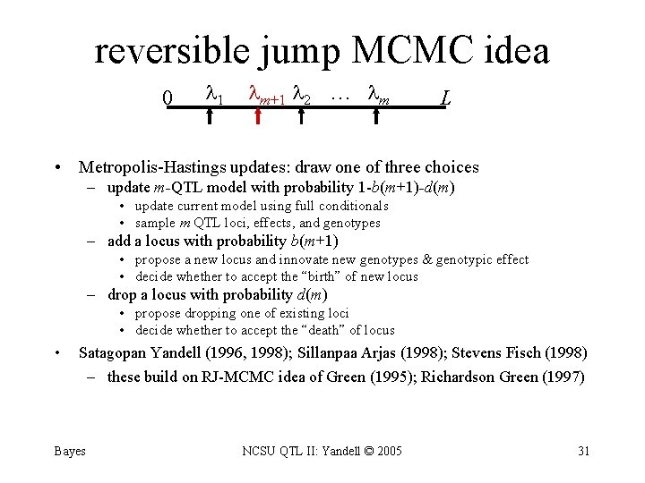
reversible jump MCMC idea 0 1 m+1 2 … m L • Metropolis-Hastings updates: draw one of three choices – update m-QTL model with probability 1 -b(m+1)-d(m) • update current model using full conditionals • sample m QTL loci, effects, and genotypes – add a locus with probability b(m+1) • propose a new locus and innovate new genotypes & genotypic effect • decide whether to accept the “birth” of new locus – drop a locus with probability d(m) • propose dropping one of existing loci • decide whether to accept the “death” of locus • Satagopan Yandell (1996, 1998); Sillanpaa Arjas (1998); Stevens Fisch (1998) – these build on RJ-MCMC idea of Green (1995); Richardson Green (1997) Bayes NCSU QTL II: Yandell © 2005 31

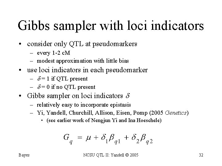
Gibbs sampler with loci indicators • consider only QTL at pseudomarkers – every 1 -2 c. M – modest approximation with little bias • use loci indicators in each pseudomarker – = 1 if QTL present – = 0 if no QTL present • Gibbs sampler on loci indicators – relatively easy to incorporate epistasis – Yi, Yandell, Churchill, Allison, Eisen, Pomp (2005 Genetics) • (see earlier work of Nengjun Yi and Ina Hoeschele) Bayes NCSU QTL II: Yandell © 2005 32