Bayesian inference J Daunizeau Brain and Spine Institute

Bayesian inference J. Daunizeau Brain and Spine Institute, Paris, France Wellcome Trust Centre for Neuroimaging, London, UK

Overview of the talk 1 Probabilistic modelling and representation of uncertainty 1. 1 Bayesian paradigm 1. 2 Hierarchical models 1. 3 Frequentist versus Bayesian inference 2 Numerical Bayesian inference methods 2. 1 Sampling methods 2. 2 Variational methods (Re. ML, EM, VB) 3 SPM applications 3. 1 a. MRI segmentation 3. 2 Decoding of brain images 3. 3 Model-based f. MRI analysis (with spatial priors) 3. 4 Dynamic causal modelling

Overview of the talk 1 Probabilistic modelling and representation of uncertainty 1. 1 Bayesian paradigm 1. 2 Hierarchical models 1. 3 Frequentist versus Bayesian inference 2 Numerical Bayesian inference methods 2. 1 Sampling methods 2. 2 Variational methods (Re. ML, EM, VB) 3 SPM applications 3. 1 a. MRI segmentation 3. 2 Decoding of brain images 3. 3 Model-based f. MRI analysis (with spatial priors) 3. 4 Dynamic causal modelling

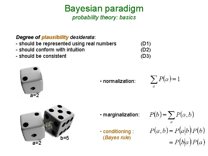
Bayesian paradigm probability theory: basics Degree of plausibility desiderata: - should be represented using real numbers - should conform with intuition - should be consistent • normalization: a=2 • marginalization: a=2 b=5 • conditioning : (Bayes rule) (D 1) (D 2) (D 3)

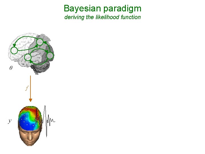
Bayesian paradigm deriving the likelihood function - Model of data with unknown parameters: e. g. , GLM: - But data is noisy: - Assume noise/residuals is ‘small’: f → Distribution of data, given fixed parameters:

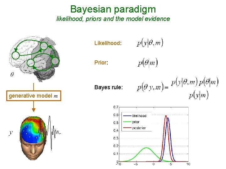
Bayesian paradigm likelihood, priors and the model evidence Likelihood: Prior: Bayes rule: generative model m

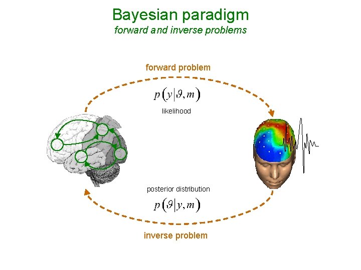
Bayesian paradigm forward and inverse problems forward problem likelihood posterior distribution inverse problem

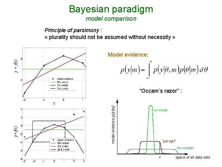
Bayesian paradigm model comparison Principle of parsimony : « plurality should not be assumed without necessity » y = f(x) Model evidence: “Occam’s razor” : model evidence p(y|m) y=f(x) x space of all data sets

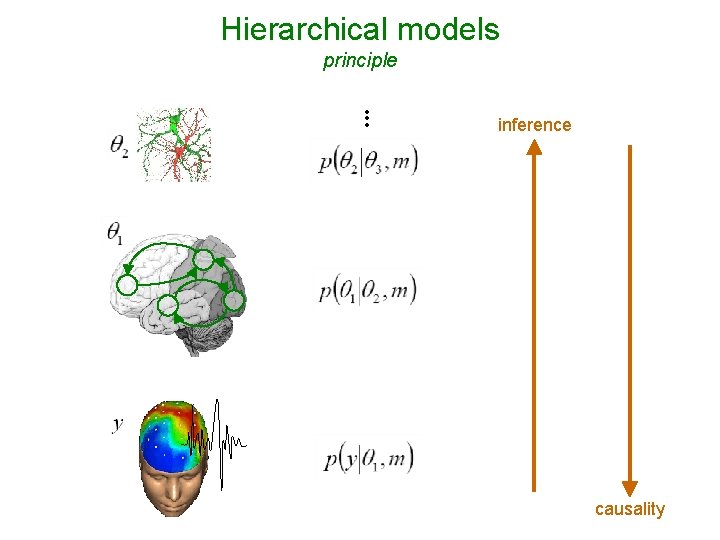
Hierarchical models principle • • • inference causality

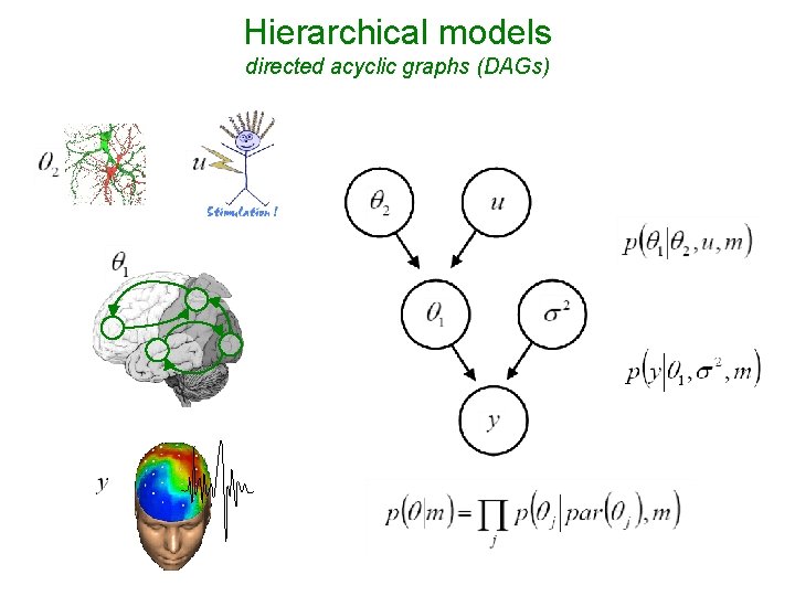
Hierarchical models directed acyclic graphs (DAGs)

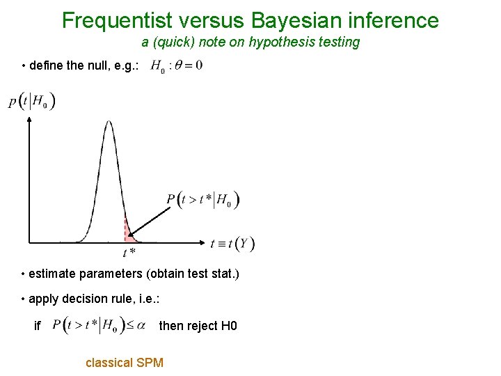
Frequentist versus Bayesian inference a (quick) note on hypothesis testing • define two alternative models, e. g. : • define the null, e. g. : • estimate parameters (obtain test stat. ) • apply decision rule, e. g. : • apply decision rule, i. e. : if space of all datasets then reject H 0 classical SPM if then accept m 0 Bayesian Model Comparison

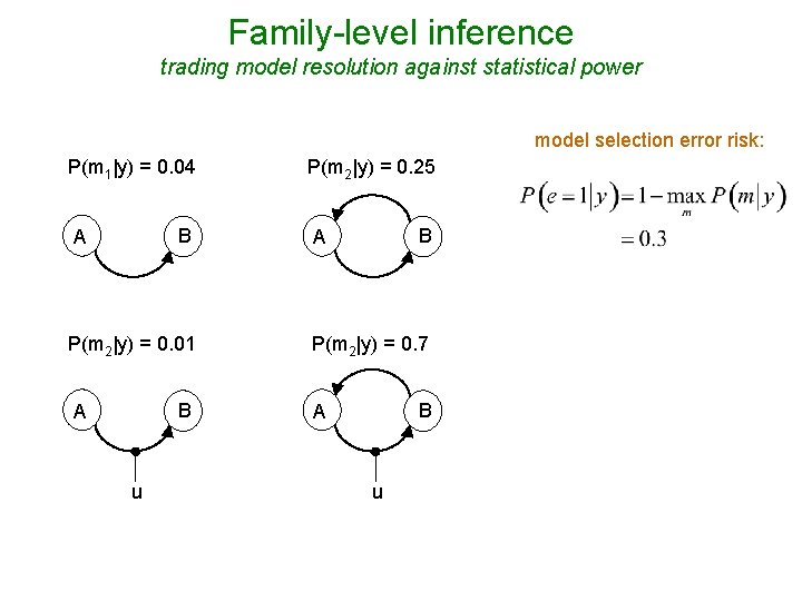
Family-level inference trading model resolution against statistical power model selection error risk: P(m 1|y) = 0. 04 B A P(m 2|y) = 0. 01 B A u P(m 2|y) = 0. 25 B A P(m 2|y) = 0. 7 B A u

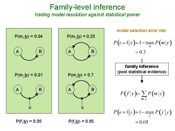
Family-level inference trading model resolution against statistical power model selection error risk: P(m 1|y) = 0. 04 B A P(m 2|y) = 0. 01 B A P(m 2|y) = 0. 25 B A P(m 2|y) = 0. 7 B A u u P(f 1|y) = 0. 05 P(f 2|y) = 0. 95 family inference (pool statistical evidence)

Overview of the talk 1 Probabilistic modelling and representation of uncertainty 1. 1 Bayesian paradigm 1. 2 Hierarchical models 1. 3 Frequentist versus Bayesian inference 2 Numerical Bayesian inference methods 2. 1 Sampling methods 2. 2 Variational methods (Re. ML, EM, VB) 3 SPM applications 3. 1 a. MRI segmentation 3. 2 Decoding of brain images 3. 3 Model-based f. MRI analysis (with spatial priors) 3. 4 Dynamic causal modelling

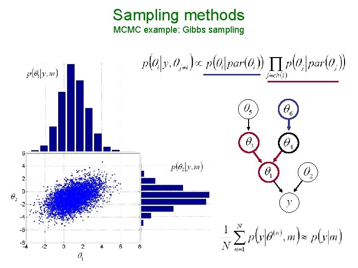
Sampling methods MCMC example: Gibbs sampling

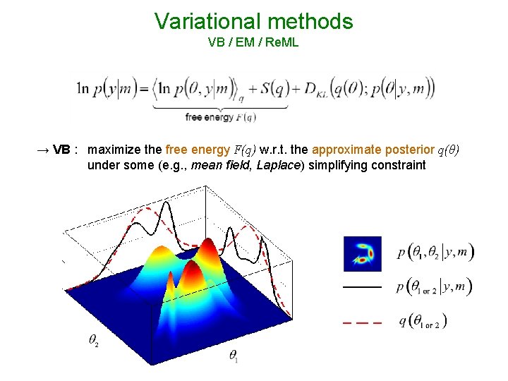
Variational methods VB / EM / Re. ML → VB : maximize the free energy F(q) w. r. t. the approximate posterior q(θ) under some (e. g. , mean field, Laplace) simplifying constraint

Overview of the talk 1 Probabilistic modelling and representation of uncertainty 1. 1 Bayesian paradigm 1. 2 Hierarchical models 1. 3 Frequentist versus Bayesian inference 2 Numerical Bayesian inference methods 2. 1 Sampling methods 2. 2 Variational methods (Re. ML, EM, VB) 3 SPM applications 3. 1 a. MRI segmentation 3. 2 Decoding of brain images 3. 3 Model-based f. MRI analysis (with spatial priors) 3. 4 Dynamic causal modelling

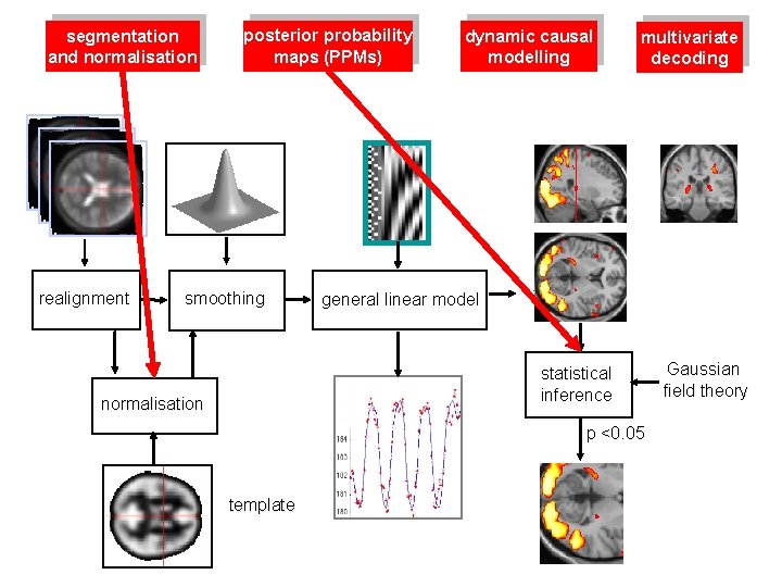
segmentation and normalisation realignment posterior probability maps (PPMs) smoothing dynamic causal modelling multivariate decoding general linear model statistical inference normalisation p <0. 05 template Gaussian field theory

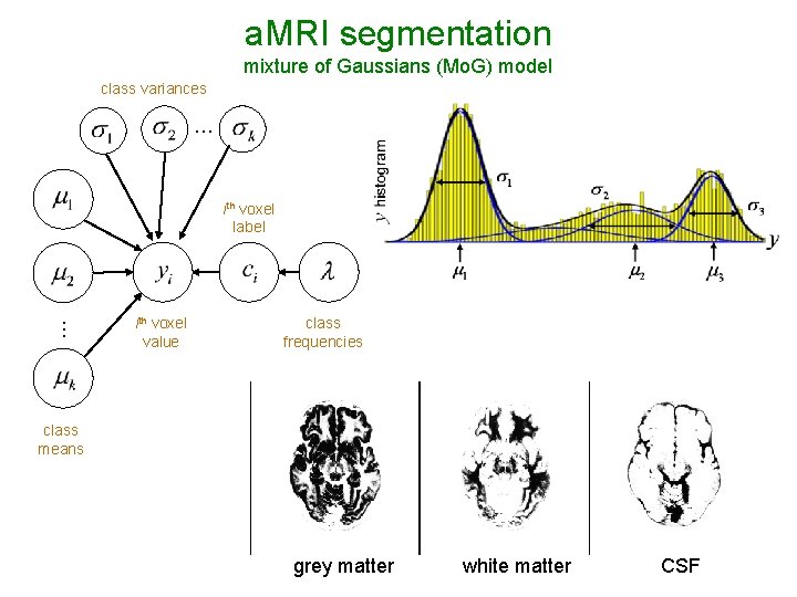
a. MRI segmentation mixture of Gaussians (Mo. G) model class variances … … ith voxel label ith voxel value class frequencies class means grey matter white matter CSF

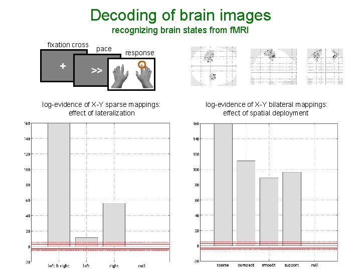
Decoding of brain images recognizing brain states from f. MRI fixation cross + pace response >> log-evidence of X-Y sparse mappings: effect of lateralization log-evidence of X-Y bilateral mappings: effect of spatial deployment

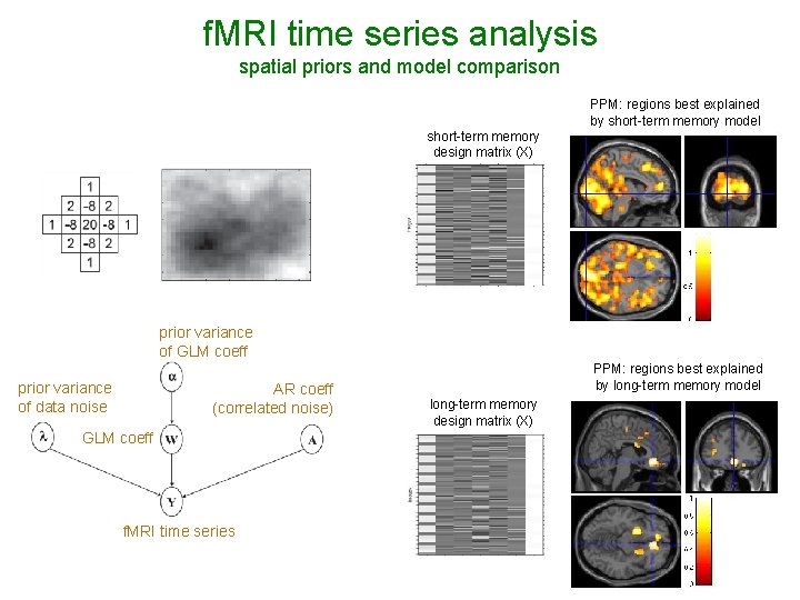
f. MRI time series analysis spatial priors and model comparison PPM: regions best explained by short-term memory model short-term memory design matrix (X) prior variance of GLM coeff prior variance of data noise AR coeff (correlated noise) GLM coeff f. MRI time series PPM: regions best explained by long-term memory model long-term memory design matrix (X)

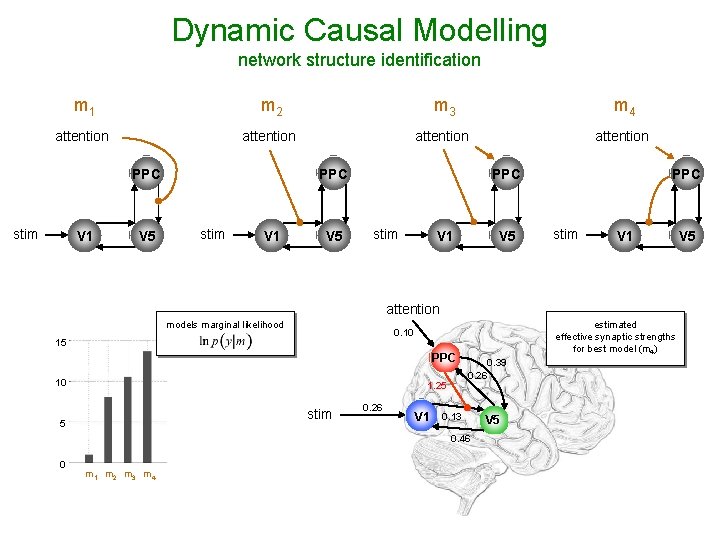
Dynamic Causal Modelling network structure identification m 1 m 2 m 3 m 4 attention PPC stim V 1 V 5 PPC stim V 1 attention models marginal likelihood 15 PPC 10 1. 25 stim 5 estimated effective synaptic strengths for best model (m 4) 0. 10 0. 26 V 1 0. 39 0. 26 0. 13 0. 46 0 m 1 m 2 m 3 m 4 V 5

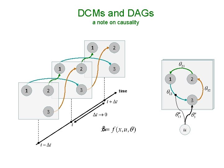
DCMs and DAGs a note on causality 1 1 2 2 3 1 1 2 3 2 time 3 3 u

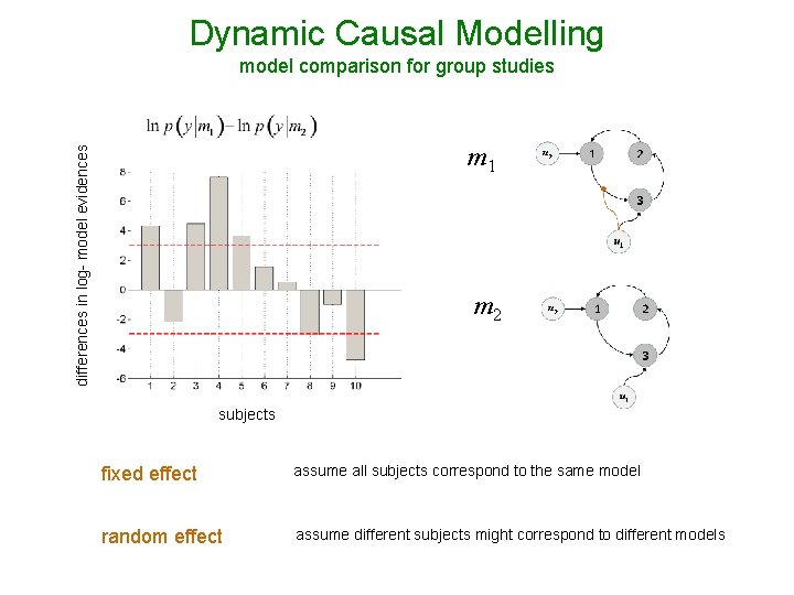
Dynamic Causal Modelling model comparison for group studies differences in log- model evidences m 1 m 2 subjects fixed effect assume all subjects correspond to the same model random effect assume different subjects might correspond to different models

I thank you for your attention.

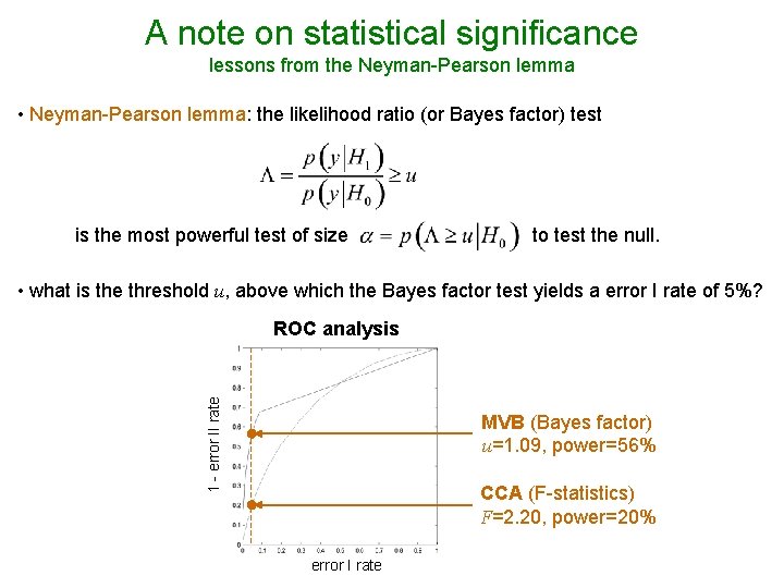
A note on statistical significance lessons from the Neyman-Pearson lemma • Neyman-Pearson lemma: the likelihood ratio (or Bayes factor) test is the most powerful test of size to test the null. • what is the threshold u, above which the Bayes factor test yields a error I rate of 5%? 1 - error II rate ROC analysis MVB (Bayes factor) u=1. 09, power=56% CCA (F-statistics) F=2. 20, power=20% error I rate