BAYESIAN INFERENCE BASED ON Extreme value Distribution STATISTICAL

BAYESIAN INFERENCE BASED ON Extreme value Distribution

STATISTICAL INFERENCE CLASSICAL INFERENCE STURACTURAL INFERENCE BAYESIAN INFERENCE

BAYESIAN INFERENCE (1) Distribution parameters are variables (2) Depends on distribution prior Which depends on previous information such as the experience of the researcher of the parameters of the distribution used other than the information in the sample

The aim of our research find a unified approach on which the researchers rely on the pre-distribution based on the known information about the distribution and therefore the results of the statistical experiment are not affected by different researchers

Distribution parameters 1 - Reliability Function R(t) For given t 2 - Cumulative Dist. Function CDF F(t) for given t 3 - Quintile Function Q(p) for given p

0 < CDF < 1 0<log Inv. Gamma<1 Change of variables Informative prior:

Non- informative prior

Type II Extreme value dist. 1 - Natural Disasters: Extreme atmospheric pressures, floods, speed of winds, Volcano eruption, Earthquakes, The tsunami 2 - Air Pollution Measurements 3 - Service Time: Pilgrimage , Friday prayer.

This Dist. Contains two Parameters: 1 - Shape parameter 2 - Scale parameter ( ) Point Estimates & Intervals Estimates & & R(t)

BAYES INFERENCE BASED ON TYPE-II PROGRESSIVELY CENSORED SAMPLE

Extreme value dist

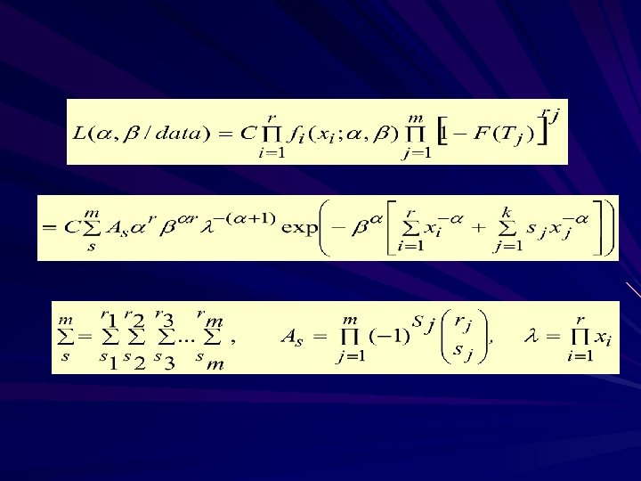
NIF. of α & β

INF. ON α & β

For intervals estimates: The credible intervals (A, B) for (say) can be found such that: OR

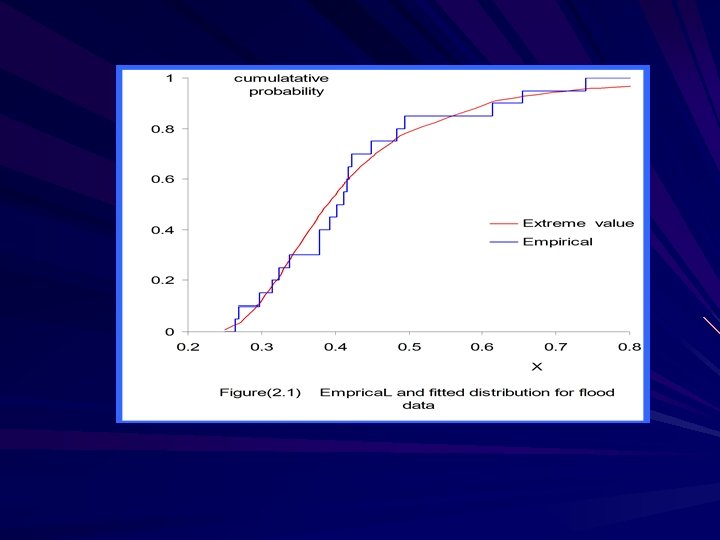
Example Consider the data given by Dumonceaux and Antle (1973), obtained of the maximum flood level (in millions of cubic feet per second) for the River at Harrisburg, Pennsylvania over 20 four-year periods (1890 -1969), which can be written in order as:

0. 265, 0. 324, 0. 392, 0. 418, 0. 494, 0. 269, 0. 338, 0. 402, 0. 423, 0. 613, 0. 297, 0. 379, 0. 412, 0. 449, 0. 654, 0. 315, 0. 379, 0. 416, 0. 484, 0. 740.

We give a rough indication of the goodness of fit for the model, due to the smallness of the sample size, by plotting the empirical cdf and the cdf of the EVD, using the maximum likelihood estimators (MLE’s) as estimates for the parameters

• In the following Table the point and interval estimates of the unknown parameters , and reliability R(t) at t=0. 3, 0. 35 and 0. 4 are calculated based on the type II Prog. censored sample.

1 - 0. 90 t NIF INF. R LL UL (2. 4302) 5. 3515 2. 7208 (2. 8981) 5. 5820 0. 3 3. 1889 (2. 4271) 5. 6159 2. 9554 (2. 8941) 5. 8495 0. 35 3. 1518 (2. 3557) 5. 5075 2. 9262 (2. 8073) 5. 7336 0. 4 3. 0017 (2. 2282) 5. 2299 2. 7885 (2. 6551) 5. 4436 0. 3037 (0. 1697) 0. 3904 0. 2974 (0. 1892) 0. 3966 0. 3031 (0. 1677) 0. 3909 0. 2964 (0. 1812) 0. 3976 0. 35 0. 3076 (0. 1665) 0. 3941 0. 3020 (0. 1792) 0. 4012 0. 4 0. 3031 (0. 1637) 0. 3909 0. 2944 (0. 1712) 0. 3976 0. 3182 (0. 4257) 0. 7439 0. 3960 (0. 4375) 0. 7710 0. 3259 (0. 4157) 0. 7481 0. 3131 (0. 4561) 0. 7692 0. 35 0. 3371 (0. 4150) 0. 7521 0. 3253 (0. 4489) 0. 7742 0. 4 0. 3411 (0. 4121) 0. 7532 0. 3293 (0. 4538) 0. 7831 NIF. INF. UL 2. 9513 NIF. INF. LL 0. 95

In the following Figures, illustration of the structural densities of the parameters and reliability are plotted, to study their behavior based on type II Prog. censored sample.

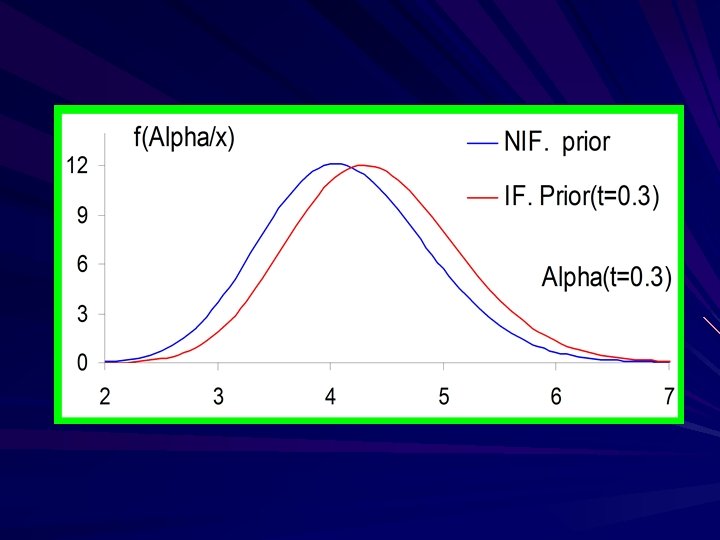
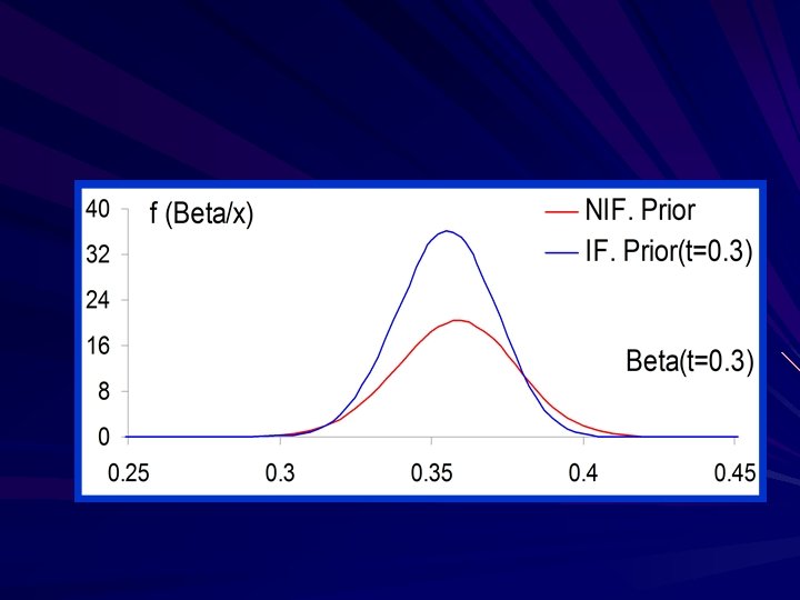
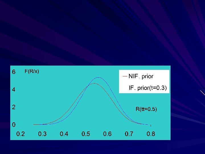
Conclusion we found the length of intervals based on the IF prior are smaller than those based on the NIF prior especially for large values of . The figures indicates that the posterior of α and β are quite symmetric, and the posterior of R is negatively skewed with a short left tail, which ensures the results.

Thank you