Bayesian gene set analysis for identifying significant biological

Bayesian gene set analysis for identifying significant biological pathways Babak Shahbaba University of California, Irvine, USA and Robert Tibshirani, Catherine M. Shachaf and Sylvia K. Plevritis Stanford University, USA Journal of the Royal Statistical Society 2011

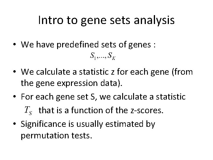
Intro to gene sets analysis • We have predefined sets of genes : • We calculate a statistic z for each gene (from the gene expression data). • For each gene set S, we calculate a statistic that is a function of the z-scores. • Significance is usually estimated by permutation tests.

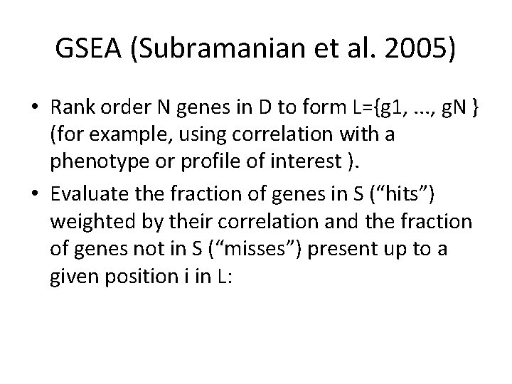
GSEA (Subramanian et al. 2005) • Rank order N genes in D to form L={g 1, . . . , g. N } (for example, using correlation with a phenotype or profile of interest ). • Evaluate the fraction of genes in S (“hits”) weighted by their correlation and the fraction of genes not in S (“misses”) present up to a given position i in L:

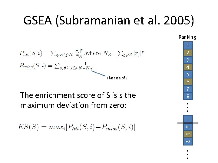
GSEA (Subramanian et al. 2005) Ranking The size of S The enrichment score of S is s the maximum deviation from zero: 1 2 3 4 5 6 7 8 i i+1 i+2 i+3

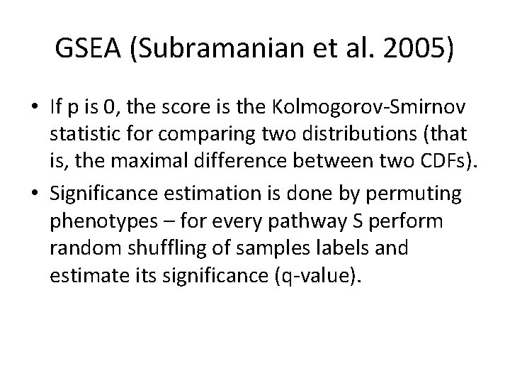
GSEA (Subramanian et al. 2005) • If p is 0, the score is the Kolmogorov-Smirnov statistic for comparing two distributions (that is, the maximal difference between two CDFs). • Significance estimation is done by permuting phenotypes – for every pathway S perform random shuffling of samples labels and estimate its significance (q-value).

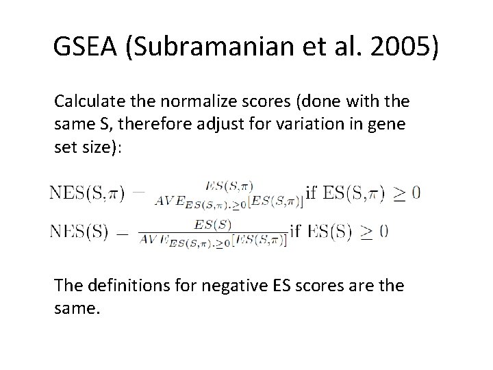
GSEA (Subramanian et al. 2005) Calculate the normalize scores (done with the same S, therefore adjust for variation in gene set size): The definitions for negative ES scores are the same.

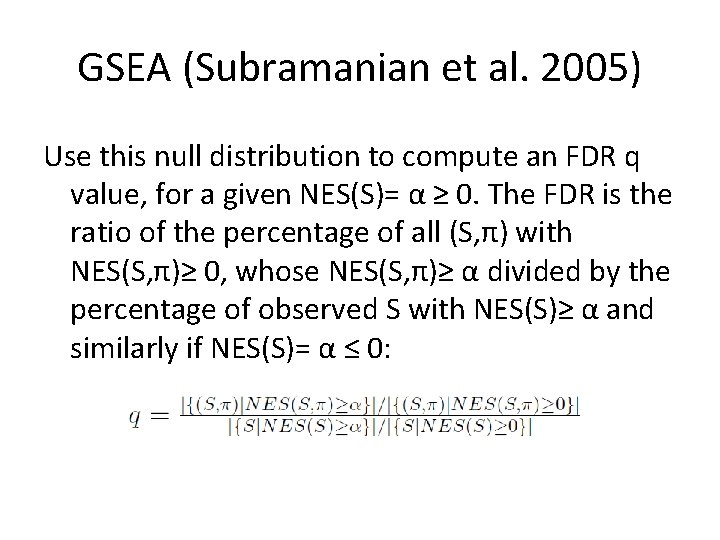
GSEA (Subramanian et al. 2005) Use this null distribution to compute an FDR q value, for a given NES(S)= α ≥ 0. The FDR is the ratio of the percentage of all (S, π) with NES(S, π)≥ 0, whose NES(S, π)≥ α divided by the percentage of observed S with NES(S)≥ α and similarly if NES(S)= α ≤ 0:

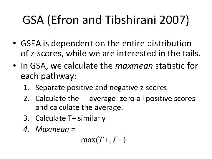
GSA (Efron and Tibshirani 2007) • GSEA is dependent on the entire distribution of z-scores, while we are interested in the tails. • In GSA, we calculate the maxmean statistic for each pathway: 1. Separate positive and negative z-scores 2. Calculate the T- average: zero all positive scores and calculate the average. 3. Calculate T+ similarly 4. Maxmean =

GSA permutations • As in GSEA, GSA use permutations on the samples labels. • However, GSA also uses estimations on random pathways: all maxmean statistics are first standardized using random pathway scores, and then significance is estimated using label permutations. • Maxmean drawback – works well especially when all genes in the pathway are up or down regulated.

Fast intro to Bayesian inference and estimation • • • Likelihood Bayes: priors and posteriors MCMC Estimation using Gibbs sampling Hierarchical Bayes models

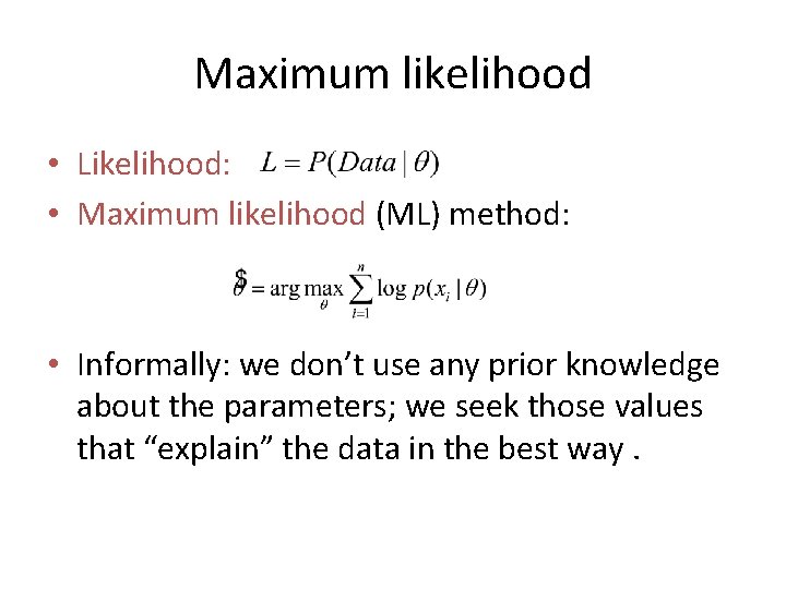
Maximum likelihood • Likelihood: • Maximum likelihood (ML) method: • Informally: we don’t use any prior knowledge about the parameters; we seek those values that “explain” the data in the best way.

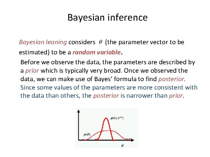
Bayesian inference Bayesian leaning considers (the parameter vector to be estimated) to be a random variable. Before we observe the data, the parameters are described by a prior which is typically very broad. Once we observed the data, we can make use of Bayes’ formula to find posterior. Since some values of the parameters are more consistent with the data than others, the posterior is narrower than prior.

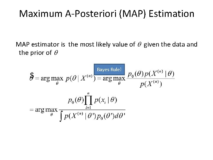
Maximum A-Posteriori (MAP) Estimation MAP estimator is the most likely value of q given the data and the prior of q Bayes Rule!

MCMC • In complex models we won’t have an analytical solution for the posterior. • Markov Chain Monte Carlo • Markov chain: a stochastic process in which the future state is independent of past states, given the current state. • Monte-Carlo: sampling based techniques for calculating integrals of the form:

MCMC • We sample different θs to calculate the desired function (average, max etc. ). • We use a Markov process to guide the sampling process so that it will mimic the posterior. If the chain satisfies several conditions then the estimator is consistent. • Popular algorithms employ random walk to guide the sampling: – Metropolis-Hastings algorithm – Gibbs sampling

Gibbs sampler If we want to calculate a property of the posterior (e. g. the mean): and we know the full conditionals then the Gibbs sampler works as follow:

Hierarchical Bayes model • A general statistical framework that can capture dependencies. • As in any Bayesian framework, a data X is dependent on a variable θ, however θ is dependent on other variable φ and so on. • So, we have a chain of priors…does it make sense?

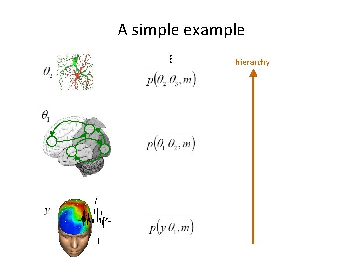
A simple example • • • hierarchy

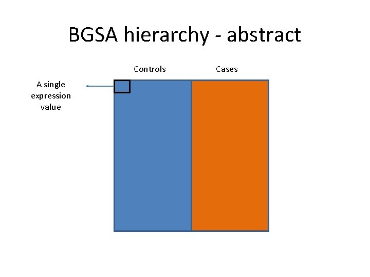
BGSA hierarchy - abstract Controls A single expression value Cases

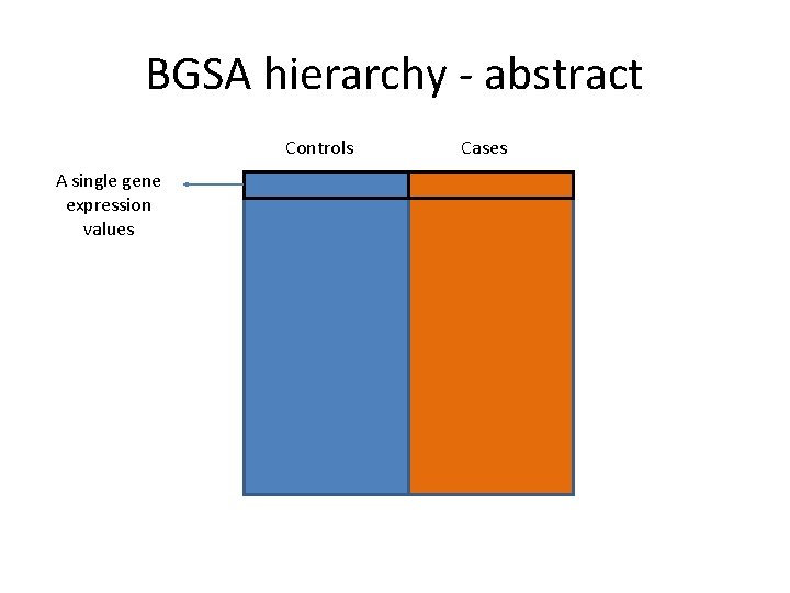
BGSA hierarchy - abstract Controls A single gene expression values Cases

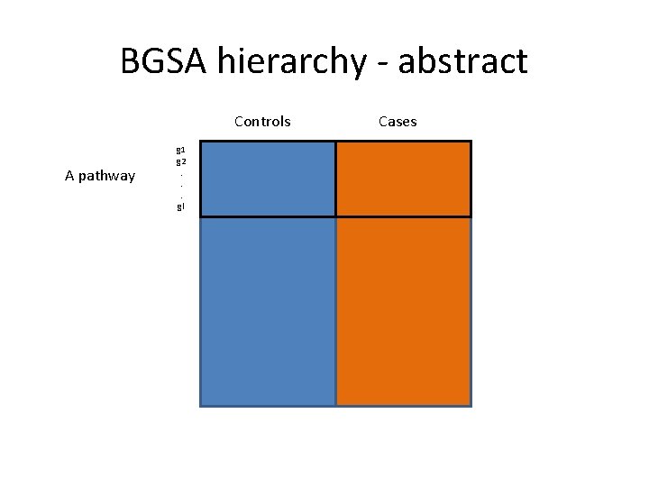
BGSA hierarchy - abstract Controls A pathway g 1 g 2. . . gl Cases

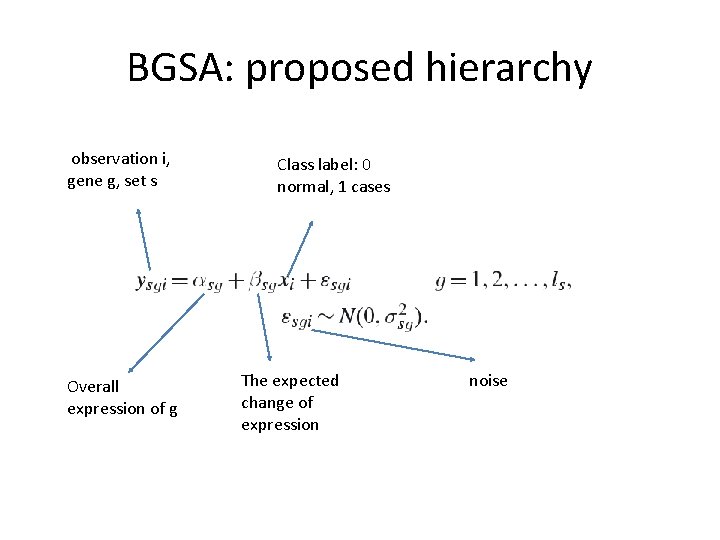
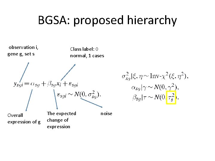
BGSA: proposed hierarchy observation i, gene g, set s Overall expression of g Class label: 0 normal, 1 cases The expected change of expression noise

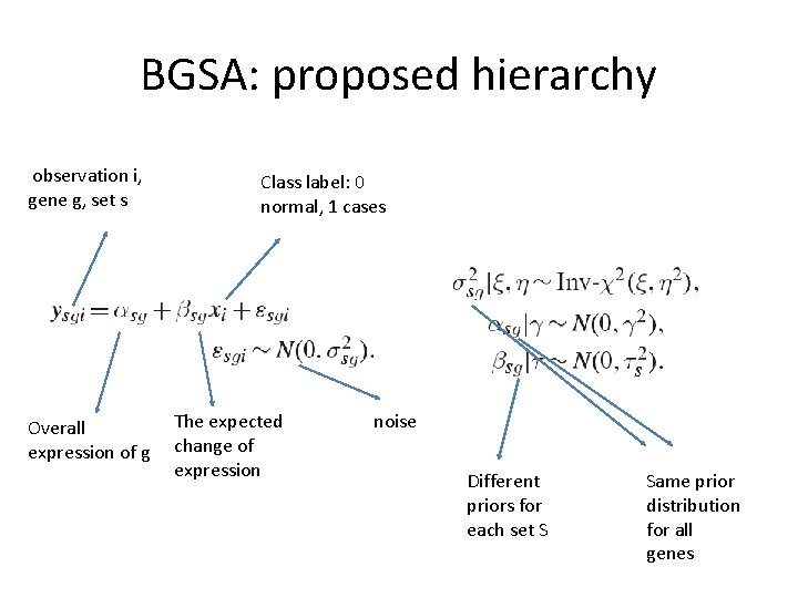
BGSA: proposed hierarchy observation i, gene g, set s Overall expression of g Class label: 0 normal, 1 cases The expected change of expression noise Different priors for each set S Same prior distribution for all genes

Inverse Chi square distribution

BGSA: proposed hierarchy observation i, gene g, set s Overall expression of g Class label: 0 normal, 1 cases The expected change of expression noise

Gene common non-informative priors • These are derived from the same common priors, we therefore select constant and wide priors (it will also ease computations): • Set • If we assume that • Then we get

The gene set statistic The role of is to adjust the distribution of gene changes in a specific pathway. If most genes in the pathway do not differentiate, it will shrink to zero.

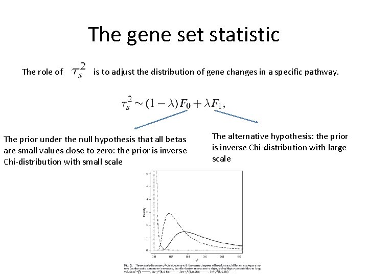
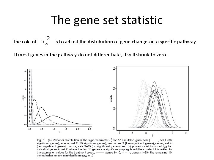
The gene set statistic The role of is to adjust the distribution of gene changes in a specific pathway. The prior under the null hypothesis that all betas are small values close to zero: the prior is inverse Chi-distribution with small scale The alternative hypothesis: the prior is inverse Chi-distribution with large scale

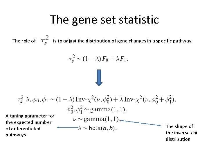
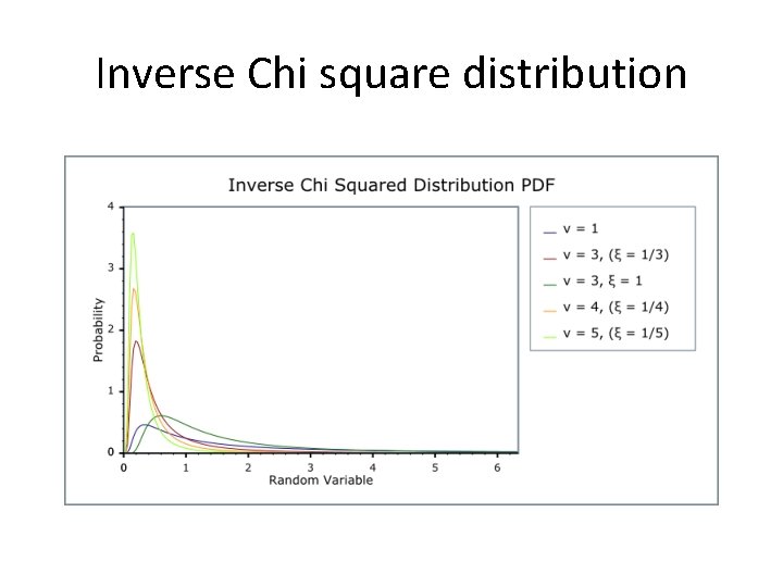
The gene set statistic The role of is to adjust the distribution of gene changes in a specific pathway. A tuning parameter for the expected number of differentiated pathways. The shape of the inverse-chi distribution

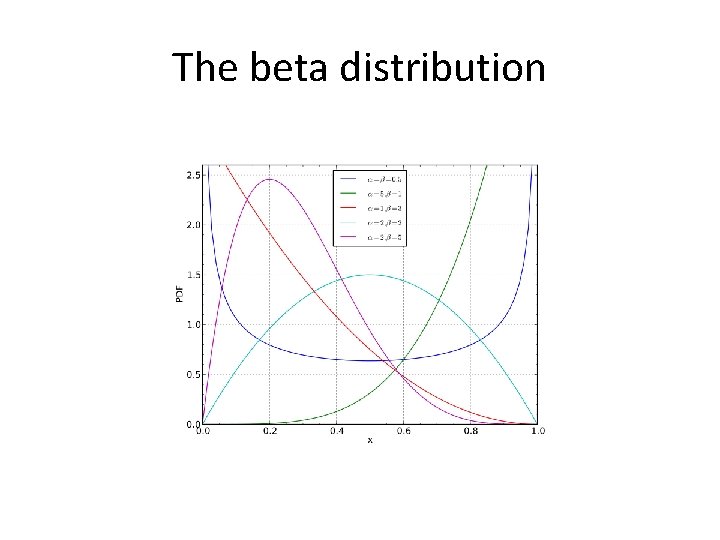
The beta distribution

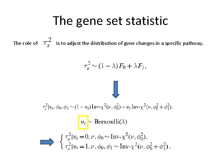
The gene set statistic The role of is to adjust the distribution of gene changes in a specific pathway.

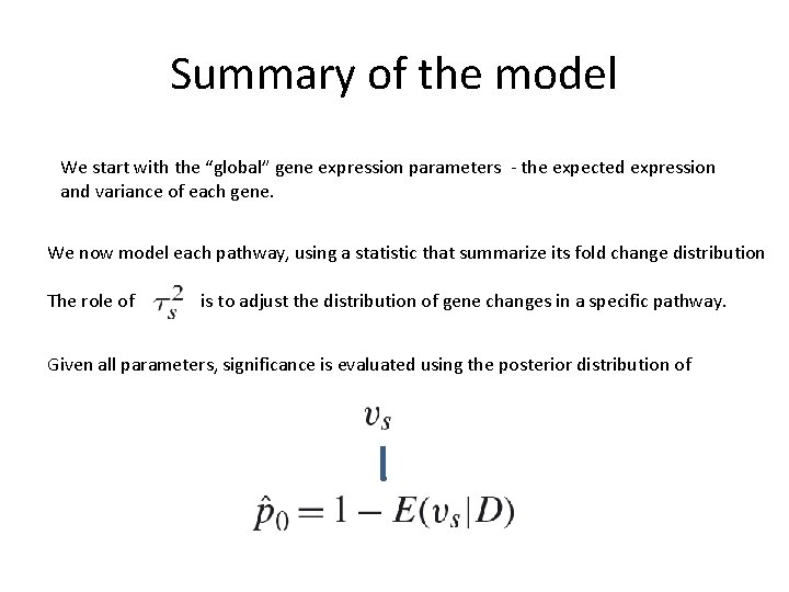
Summary of the model We start with the “global” gene expression parameters - the expected expression and variance of each gene. We now model each pathway, using a statistic that summarize its fold change distribution The role of is to adjust the distribution of gene changes in a specific pathway. Given all parameters, significance is evaluated using the posterior distribution of

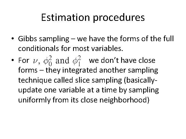
Estimation procedures • Gibbs sampling – we have the forms of the full conditionals for most variables. • For we don’t have close forms – they integrated another sampling technique called slice sampling (basicallyupdate one variable at a time by sampling uniformly from its close neighborhood)

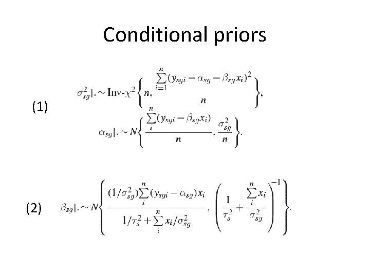
Conditional priors (1) (2)

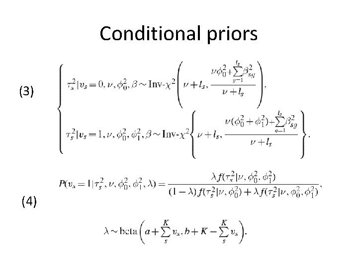
Conditional priors (3) (4)

Results • Used the p 53 data that GSEA used: cancer cell line analysis of p 53 mutant (n=33) vs. wt (n=17). • Used 522 pathways available from MSIGDB.

Simulated data • 100 repeats of: – Randomly down-sample the p 53 data matrix to have 10 -20 samples (overall) – Randomly shuffle the genes in the 522 pathways – Randomly select 5 gene sets and reallocate the top 20 differential genes among them. • Evaluate each method in terms of ROC score: for each simulation rank all 522 “pathways” and treat the 5 chosen gene sets as “positives”.

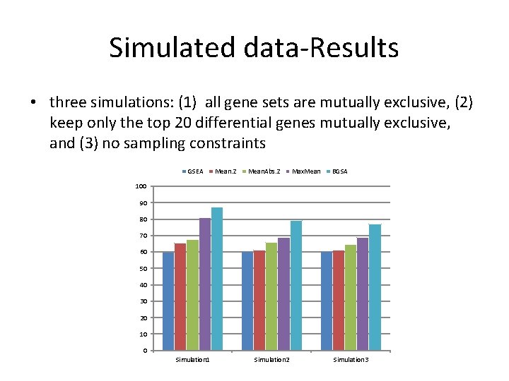
Simulated data-Results • three simulations: (1) all gene sets are mutually exclusive, (2) keep only the top 20 differential genes mutually exclusive, and (3) no sampling constraints GSEA Mean. Z Mean. Abs. Z Max. Mean BGSA 100 90 80 70 60 50 40 30 20 10 0 Simulation 1 Simulation 2 Simulation 3

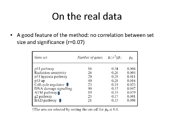
On the real data • A good feature of the method: no correlation between set size and significance (r=0. 07)

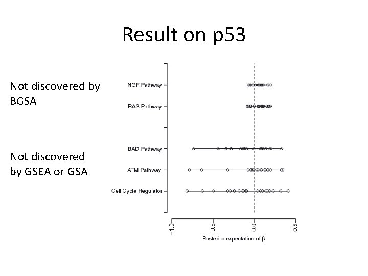
Result on p 53 Not discovered by BGSA Not discovered by GSEA or GSA

Comments • It is not clear if GSEA with ranking by absolute z-scores provides similar results. • They do not mention the significance level used for GSA and GSEA. • Simulation is biased towards creating random gene-sets that are “mixed” in terms of the number of up- and down- regulated genes. • GSA seems simple and outperforms GSEA.