Bayesian Decision Making Charles S Tapiero Individual Bayes

Bayesian Decision Making Charles S. Tapiero

Individual Bayes decision making is based on a personal interpretation of probability, quantifying what may seem subjective assessments of events in terms of quantitative terms regarding the uncertainty underlying the problem

Bayesian analysis represents a rational procedure that uses all the data which is relevant and available. It provides an economic approach to evaluating alternatives based on prior judgment formulated in terms of the data initially available.

Decision Trees • Often, it is convenient to represent the potential scenarios that uncertainty can unfold through graphical means. To do so, we use Decision Trees, which is a simple graphical form to represent decision problems under uncertainty. In a DT we represent graphically the linkages between a decision and its consequences.

• Different outcomes and costs are valued differently, expressing a decision-maker's preference. In this problem, there are several decisions and events, each of which depends on the other. To represent the sequence of decisions and their events, it is useful to express the problem in a so-called 'decision-tree' format. This is simply a diagrammatic depiction showing the various actions, outcomes and sources of uncertainty, and the order in which decisions and outcomes happen. How do we construct and "grow" such decision trees? First we organize decisions and their events following their natural sequence. For convenience, we use a square to denote a decision point, out of which a number of outgoing lines equals the set of alternative decisions that may be taken, as shown above. Now, since each decision is followed by an event, (which is known only in terms of the states of nature and their probabilities at the decision time), we can represent the sequence of decision-events and their probabilities by a decision-tree diagrammatic relationship. The decision-tree where we can observe that the outcomes are represented as branches which evolve from the decision point.

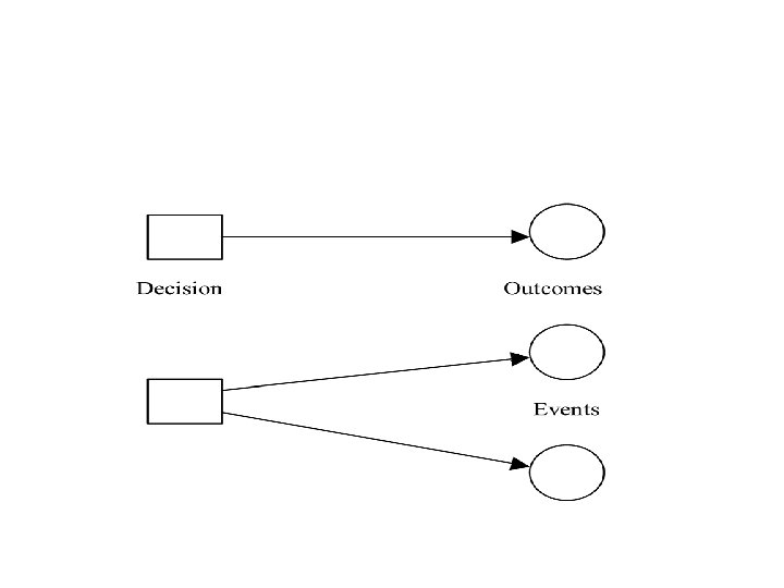
• Decision trees may involve more than one decision point. In particular, decisions may depend on outcomes that are uncertain at a given decision time. This leads to general "multi-stage" decision trees which are more difficult to analyze. A two-stage decision tree problem of special importance consists in linking information acquisition together with the actual decision making problem being entertained. Say that information relating to a given problem can be acquired. Then the decision tree format can be expanded. Such a decision problem would involve the following phases

Phase I: Data Collection Stage Prior Posterior Information State Collection Strategic Decisions Conditional Consequences State Phase II: Decision and Evaluation Stage

• Phase 1: Collect information or not and if so, how much (such as survey data) • Assess the conditional consequences of such data on the uncertainty faced by the DM while reaching a strategic decision • Phase 2: Reach a strategic decision • Assess the conditional consequences of this decision not only in terms of potential and realizable outcomes but also in terms of the costs of the strategic decision and the costs of collecting the information use din reaching the strategic decision.

• Although these problems can still be analyzed, they are a little more difficult. This will be done subsequently. As long as some uncertainty remains in a decision problem it can be treated by specifying a 'criterion of choice'. That is, the manager specifies a rule through which he will select an action, among those available and take account of the uncertainties. Such a rule will express an attitude toward the risk inherent in the problem. What are these rules. These are the criteria of choice under uncertainty we study below.

Decision Criteria • • • The expected value (or Bayes') criterion Principle of Insufficient Reason The Minimax (Maximin) Criterion The Maximax (Minimin) Criterion The Hurwicz criterion The Minimax Regret or Savage's Regret Criterion

The expected value (or Bayes') criterion. • This consists of selecting the largest expected monetary value (denoted by EMV), among a number of well defined alternatives. The EMV is a special case of the more general expected utility criterion we shall present subsequently. If the matrix entries are opportunity losses (OL), we compute the EOL or Expected Opportunity Loss and choose the alternative with the least value. Invariably, when either the EMV or EOL criterion is used, the same decision is reached. This is not a mere coincidence but an important property of decision theory.

• Preference is expressed by outcomes weighed by their corresponding probabilities. We sum them to choose that action with least (in case of costs) or most (in case of profits) weighted sum, or expected value. For monetary values, the resulting criterion is called EMV, or the Expected Monetary Value. The criterion is then to select the strategy that yields the greatest EMV. When the table is one of OL, or Opportunity Loss, we compute the EOL or Expected Opportunity Loss. The criterion is then to select the strategy that yields the least EOL. Invariably, when either the EMV or EOL criterion is used, the same decision is reached. This is not a mere coincidence but an important property of the Bayes decision rule structure.

Principle of Insufficient Reason The Laplace Criterion, named after Laplace, the famous French mathematician who postulated the "Principle of Insufficient Reason" for decision problems under complete ignorance. This principle states that when we do not know what are the probabilities of the states of nature in a given problem, we can assume that all probabilities are equally likely, reflecting a state of utmost ignorance. Thus, to compute a decision objective we apply the expected criterion as if all states of nature were equally likely! The "idea" behind this principle is that we adopt a distribution for the states of nature which assumes the least information and this distribution consists of equal probabilities.

The minimax criterion • It is used when we wish to adopt an attitude of abject pessimism and to assume that the worst will happen. It does not allow us to incorporate any judgments we may have on the relative likelihood of the various uncertain events however.

For the Motivated Reader* • Minimax optimality has been applied to many problems in operations research. For example, let be a vector of decision variables and let • be costs generated under a set of S “scenarios”. Further, let be a constraint se with

Assume that these are differentiable functions, then the general minimax problem can be stated as follows: If this problem has a finite minimax solution then it may be equivalently expressed as the nonlinear programming problem:

where If g is pseudo-convex then the solution to this problem exists.

The Maximax Payoff (or the minimin cost) • This is also called the optimist criterion. It is based on the belief that the most convenient state will occur.

The Hurwicz criterion • Here a coefficient of optimism is used. • Assuming that payoffs are used, we combine the optimistic and the pessimistic criteria as follows. • Hurwicz Criterion= a [largest payoff] + • (1 -a)[smallest payoff] • If it is a cost problem, we have • Hurwicz Criterion= a[smallest cost] + • (1 -a) [Largest Cost]

The Minimax Regret or Savage's Criterion : Ex-post, unlike ex-ante optimization, is reached once information is revealed and uncertainty is resolved. Each decision has then a regret which a decision maker will seek to minimize. The cost of a decision’s regret represents the difference between the ex-ante payoff that would be received with a given outcome compared to the maximum possible ex-post payoff that would be received with a given outcome compared to the maximum possible ex -post payoff.

Savage, Bell as well as Loomes and Sugden pointed out the relevance of this criterion to decision making under uncertainty. This criterion seeks to select an act by minimizing the regrets (i. e. the opportunity losses considered earlier) associated with the actions. Specifically, assume that we select an action (decision) and some event results. The decision-event combination generates the payoff table, a conditional consequence which is the payoff. When this occurs, we may "regret" the decision, for it is possible that we could have done better! This is the opportunity profit, which is a loss in fact, since we could have made a profit but we did not!)

If this decision were reversible (i. e. we have some flexibility) then it might be possible to compensate (at least partially) for the fact that we took, posteriori, the "wrong" decision. If there is nothing that we could aposteriori, the decision regret should have been considered in our initial computations when we were considering which decision to take. For example, say that we expect the demand for a product to grow significantly, and as a result we decide to expand the capacity of our plants. In fact however, this expectation for demand growth does not materialize and we are left with a large excess capacity and are unable to reduce capacity except at a substantial loss. What can we do then, except regret our decision! Similarly, assume that we expect peace to come on earth and decide to spend less on weapons development. Optimism, however wanted may unfortunately be not justified and instead we find ourself facing a war for which we may be ill-prepared. What can we do? Not much, except regret our decision.

The minimax regret (also called the savage regret) criterion, then, seeks to minimize the regrets we may have in adopting a decision. What would this regret be? Basically it is defined by, Regret = Best payoff received a-posteriori less the payoff actually received

The Payoff Table: A Tool of Analysis

Decision Tables • A. 1 Identify the alternative courses of action, which are variables we can control directly, when • a. 1: there must be at least two or more alternatives • a. 2: alternatives are mutually exclusive • a. 3: alternatives are collectively exhaustive

• B. Consider all possible and relevant states to a problem define by, (b. 1): each state represents one event that can occur. (b. 2): each state may itself be defined in terms of multiple other states (b. 3): states represent events which are mutually exclusive (b. 4): states are collectively exhaustive ( b. 5): one and only one state will actually result. C. Assign to each state a probability of occurrence. This probability should be based on the information we have regarding the problem and since states are mutually exclusive and collectively exhaustive, these probabilities (summed over all states) should equal to one. D. Consider all the possible conditional consequences.

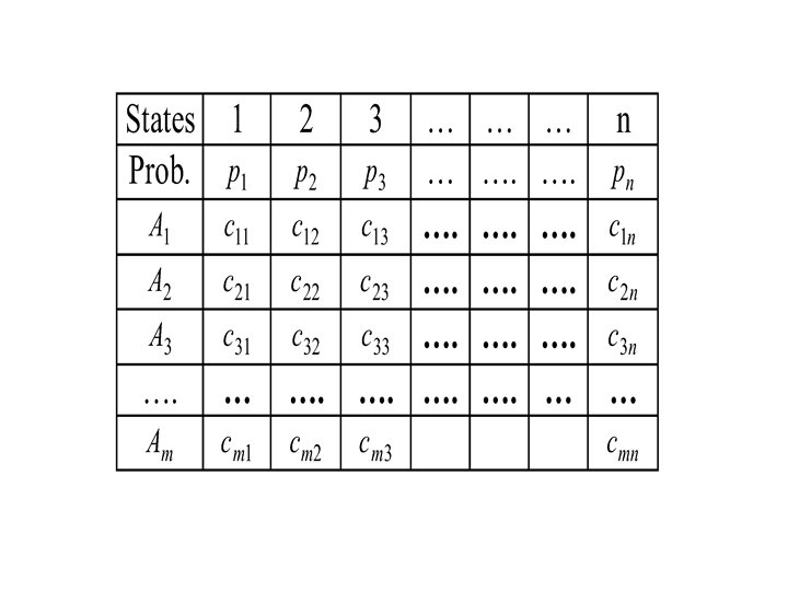
The Opportunity Loss Table:

Problem: • The buyer of a used car may have three alternatives when purchasing a car. First, accept the car as is, take the car to a special checkup and buy a service contract or warranty over a given period of time. The car may, however be in two conditions, "good" or "bad". The conditional consequences, corresponding to each "acts""states" combination are however, the car price less the costs sustained under each of the "acts" selected. Construct the decision table of such a problem.

Problem : Cash Management • Cash management consists in managing short term flow of funds in order to meet a potential need or demand for cash. Cash is kept primarily because of its need uncertainty in the future. As a result, this is essentially a problem of decision making under uncertainty. Assume, for example, that a publisher has the following needs for money:

(1) What are the potential courses of action that are faced by the book publisher (in 100 its)? (2) What are the problem states? and their probabilities? (3) What are the conditional costs if the bank rate is 20% yearly

The Criteria

• The cost of uncertainty is the expected opportunity loss of the best possible decision under a given probability distribution while the cost of irrationality is the amount by which the expected opportunity loss of the chosen decision exceeds the cost of uncertainty under a given probability distribution

• • • EPPI = EMV + EOL EPPI= EMV* + EOL* EVPI = EPPI - EMV* EVPI - C>= 0 EVPI-C= EPPI-EMV* -C=EOL* -C EVSI = EMV** - EMV*

Problem: Options • An option is a contract about an asset (securities, bonds, commodities, currencies etc. ) which confers the right to buy or sell the asset within a given time period subject to certain conditions. There are many types of options, which are used in finance. The example we shall consider refers to a European Call Option, which is the option to buy, say, a stock at a certain price (called the strike price) and at a certain time, called the maturity date (as opposed to an American option where the right to buy is conferred over the whole time interval until its maturity date). The example treated here uses only some of the ideas implied in the buying of options. Imagine a speculator whose stockbroker proposes the following investment deal:

• (i) Buy 100 shares of IBM at the current price of $75, which will pay a dividend of $10 per share at the end of the year. The cost of money during this year (which is the interest earned if we were to keep this money in the bank) is 5%. • • (b) Alternatively, with cash in hand of $7500, wed may purchase stocks at the end of the year. During this year, the money will be "parked" in the bank, yielding a 5% current interest. Of course, in this instance, the price of the IBM stock at the end of the year is uncertain

• A third alternative consists in buying instead $7500 worth of options. The option, as currently listed in the market. This mean that in a year (the option maturity date) we will be able to buy as many shares as we own options at a price of $80 (the strike price). The cost of an option, also called the premium, is $15. In other words, in order to purchase the right to buy an IBM share for $80 in one year, regardless what the IBM share price will be, we are asked to pay $15 (including commission). In addition, a study of IBM share prices, recently completed has made the following predictions regarding the IBM share prices next year. These are given by the following probability distribution. On the basis of this information, answer the following questions,

• • (a) How many options should we buy ? (b) What are the alternatives? (c) What are the states of nature for the problem? (d) What are the conditional consequences associated with each decision alternative • (e) Represent the decision tree format • (f) Represent the problem's payoff table • (g) Represent the problem's opportunity loss table

Computer Aided Solutions Decision problems can of course be resolved using the computer once they are well formulated and expressed in a Table or Decision Tree format. For this purpose there are various computer programs which can be used. Below, we consider a numerical example, summarizing all of the objectives stated above. Consider an investment problem with the following payoff tables and the following probabilities: Probabilities States of Nature Do not invest Invest 0. 15 Success 0 2, 600, 000 0. 85 Failure 0 -400, 000

Decision Analysis: INVESTMENT PROBLEM MAXIMAX Alternative ALTERN 1 ALTERN 2 Payoff 0. 00 2600. 00 * MAXIMIN Alternative ALTERN 1 ALTERN 2 Payoff 0. 00 * -400. 00

MINIMAX REGRET Alternative Payoff Regret ALTERN 1 2600. 00 ALTERN 2 400. 00 * EQUALLY LIKELY Alternative Mean Payoff ALTERN 1 0. 00 ALTERN 2 1100. 00 * Criterion MAXIMAX MAXIMIN MINIMAX REGRET EQUALLY LIKELY Decision ALTERN 2 ALTERN 1 ALTERN 2

PROBABILISTIC ANALYSIS EXPECTED VALUE Decision STATE ALTERN 1 2 0. 8500 State STATE Prob Payoff Prob*Payoff 1 0. 1500 0. 00 Expected Payoff STATE ALTERN 2 2 0. 8500 0. 00 STATE 1 0. 1500 2600. 00 -400. 00 -340. 00 Expected Payoff 50. 00 EXPECTED VALUE - SUMMARY REPORT Decision ALTERN 1 ALTERN 2 Optimal Decision: ALTERN 2 Expected Payoff 0. 00 50. 00 * 390. 00

Expected Value of Perfect Information State STATE 1 2 Prob Decision 0. 1500 ALTERN 2 0. 8500 ALTERN 1 Payoff 2600. 00 Prob*Payoff 390. 00 Expected Payoff with Perfect Information. . . Expected Payoff Without Perfect Information Expected Value of Perfect Information. . . 340. 00 390. 00 50. 00

Bayesian Decision Theory Data for period Prior distribution Bayes Mechanism Delay Posterior distribution

The conditional probability

Example: Say that an insured faces a risk which is given by the following • where "p" is the probability that an accident occurs and "X" is the size of such an accident. The probability is assumed to be distributed by a Beta probability distribution with parameters "r" and "s", or:

As accident-no-accident information is revealed, the accident probability distribution is revised by the insured and insurer as well (who use this probability to determine the size of the premium the insured has to pay). If an accident occurs, then, the bernoulli-beta process yields a posterior beta distribution with parameter B(1+r, s). However, if no accident occurs, then the posterior distribution is also beta but it is given by the following parameters B(r, 1+s). In this sense, the updating scheme can be represented by the Beta distribution B(r+q, 1 q+s), q=1, 0.

Problem : Producing for Local Markets or Export? • A manufacturer of tomato paste has traditionally concentrated its marketing effort in local markets only. Today, it is told that it might benefit and increase its profits even more if it were to export as well. Its production level is fixed at 1000 boxes of tomato paste per week. The problem it faces today is, should it divert some of its production to export and if so how much? The cost of each tomato paste box is $100 while its selling price in the local market is $150; if it were to export, the selling price of a box would be $200. Additionally, there is a surcharge of $25 per box to account for transportation, insurance, legal and other fees which are associated to exports. If the manufacturer sells its output in the local market, sales can be 500 or 1000 boxes with respective probabilities 0. 4, 0. 6.

• At the end of each week, the manufacturer tomato paste is taken off the shelf and sold at a discount of 20% to the army. If the manufacturer exports its tomato paste, it may encounter competition, so that demand may be 0, 500 or 1000 boxes. The probabilities of such demands are. 4, . 4 and. 2, respectively. In export markets, unsold tomato paste boxes at the end of the week are a total loss. On the basis of this information we are asked to decide whether or not we should export, and if we do not export, how much of the output should be sold on the local market. Assuming that Production and Marketing

• Managers communicate with each other, and production is at capacity, what can marketing recommend regarding the planning of tomato paste production capacity? Should the production capacity be expanded, be reduced, or be maintained at its current level? Use both the Table and the Decision Tree Format to answer these questions. Do not solve this problem at this time but formulate it in a decision tree format and in a Table format. Assume that all production decisions are made in units of 500's.

Reproducible Processes, Normal Distribution • For some processes, it turns out that the prior and the posterior distribution are of the same form! That is, instead of writing the Bayes recursive equation above, which is difficult to compute, it is possible to represent just the evolution of the moments of these distributions in terms of the sample information collected, which is of course much simpler and just as revealing. • Since most actions and measurements are taken on the basis of moments (parameters), it is not necessary to remember the probability distributions but only the equations tracing the evolution of such parameters. In such condition, it is said that it is a reproducible process.

• Consider again the problem considered regarding the estimate of sales. Assume at present that the probability distribution of the prior sales estimate has a normal distribution with mean =480 and variance =31600. That is if s denotes the state, which represents (approximately, since the normal distribution can theoretically have negative values) a sales level, then the probability density associated with selling s is given by the well known distribution, ìï (s - m )2 üï 1 0 = P ( s ) = C 0 exp í; C ý 0 s 02 ïþ ïî s 0 2 p

• Similarly we have contracted a market research firm to inform us that on the basis of its research, what sales are likely to be equal to. • This firm's estimates have in the past proved to be right some of the time and wrong some of the time. In fact, assume that such an estimate has a variance of 20, 000 as given earlier (for the discrete distribution). • In other words, the probability distribution of the estimate P(x/s) has a normal probability distribution with mean equaling the true sales level s and variance 20000. That is, x=s+e where e is the error term in the sales estimate having a mean zero and variance 20, 000. Since

• Using Bayes theorem for updating the distribution, and noting the fact that these are continuous probability distributions, we have • And in terms of meand variances, we have the recursive equation

• In other words if then

• In other words, assuming that the firm forecast is x=500, inserting the numerical data given for this example, we obtain a posterior probability distribution for the sales estimate that has a mean and variance which are obtained by solving, 1 s 12 1 = 31 m 1 =5923 1 + 20000 =12248

Generally

Selecting a Sample Size Prior to reaching a decision you may feel that additional information might be beneficial. In this instance, the question we may have to deal with is, how much information should we collect. Practically, if we were to collect a sample data, this decision may take the form of selecting an appropriate sample size. A simple approach to this problem consists of determining the effects of the number of samples on the variance of the data collected.

Define the average of the sample by, Applying recursively,

Through these moments we can estimate the value of information. On the basis of this value we can select the sample size. For example, if we were to let V(n) be the value of information, expressed as a function of the sample size n and if the cost of each sample is c, then the sample size will be determined by solving the following maximization problem, which consists in finding that sample size n which yields the largest next value (value V(n) less the sampling cost cn).

(Paroush and Venezia 1979) A regret example Consider a price-taking firm facing an uncertain demand x which is equal the firm's supply (assuming it holds no inventories and satisfies demand. Let p be the unit price and c(x) the production cost. The firm's profit is thus: The optimal quantity supplied is then a function of price and given by: The optimal profit and its regret are then given by:

of course, minimizing the regret will be equivalent to maximization of profits Now assume that there is a utility value given by with the following properties,

When prices are random, then optimization results are quite different. Then, Paroush and Venezia show that the optimal decision is a function of the utility second order derivatives. In this case, there is particular value to taking actions which will reduce the amount of regret the decision maker may be confronted with.