Bayesian ANOVA Or how to learn what you
Bayesian ANOVA Or how to learn what you know all over again but different

Where we're going �History of ANOVA �The Math of ANOVA �Bayes Theorem �Anatomy of Baysian ANOVA �Compare and Contrast! �Rumble in the Jungle: Advantages of Bayes �Real World 13: Genotype and Frequency Dependence in an invasive grass.
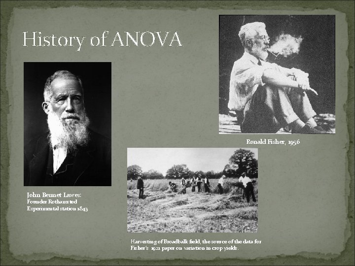
History of ANOVA Ronald Fisher, 1956 John Bennet Lawes: Founder Rothamsted Experimental station 1843 Harvesting of Broadbalk field, the source of the data for Fisher’s 1921 paper on variation in crop yields.
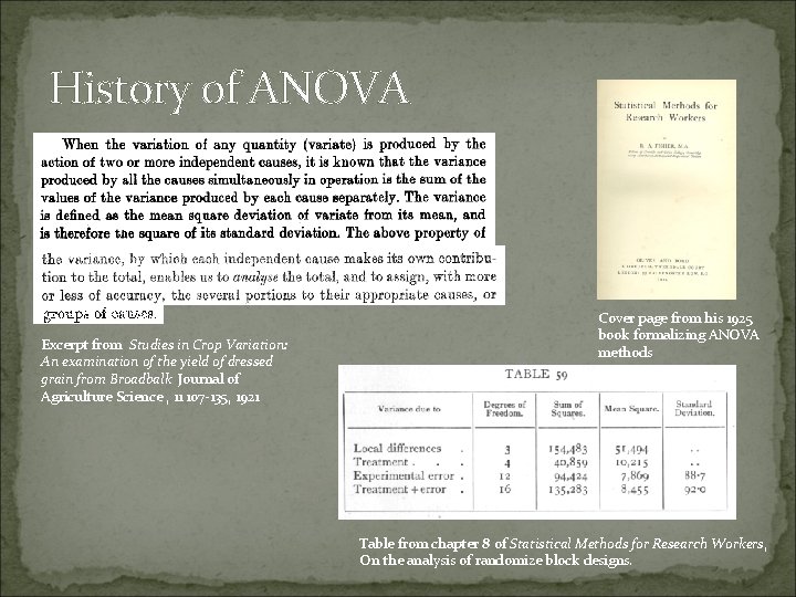
History of ANOVA Excerpt from Studies in Crop Variation: An examination of the yield of dressed grain from Broadbalk Journal of Agriculture Science , 11 107 -135, 1921 Cover page from his 1925 book formalizing ANOVA methods Table from chapter 8 of Statistical Methods for Research Workers, On the analysis of randomize block designs.

Where we're going �History of ANOVA �The Math of ANOVA �Bayes Theorem �Anatomy of Baysian ANOVA �Compare and Contrast! �Rumble in the Jungle: Advantages of Bayes �Real World 13: Genotype and Frequency Dependence in an invasive grass.
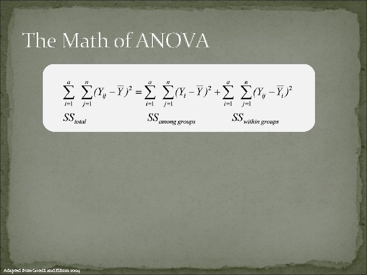
The Math of ANOVA Adapted from Gotelli and Ellison 2004
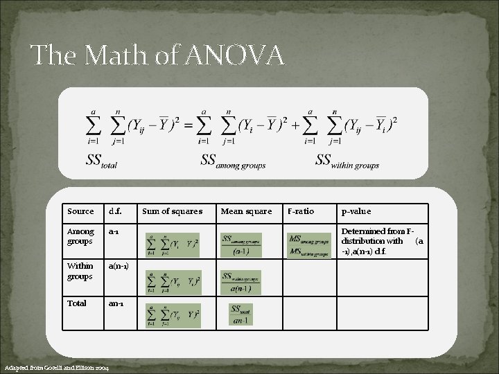
The Math of ANOVA Source d. f. Among groups a-1 Within groups a(n-1) Total an-1 Adapted from Gotelli and Ellison 2004 Sum of squares Mean square F-ratio p-value Determined from Fdistribution with (a -1), a(n-1) d. f.
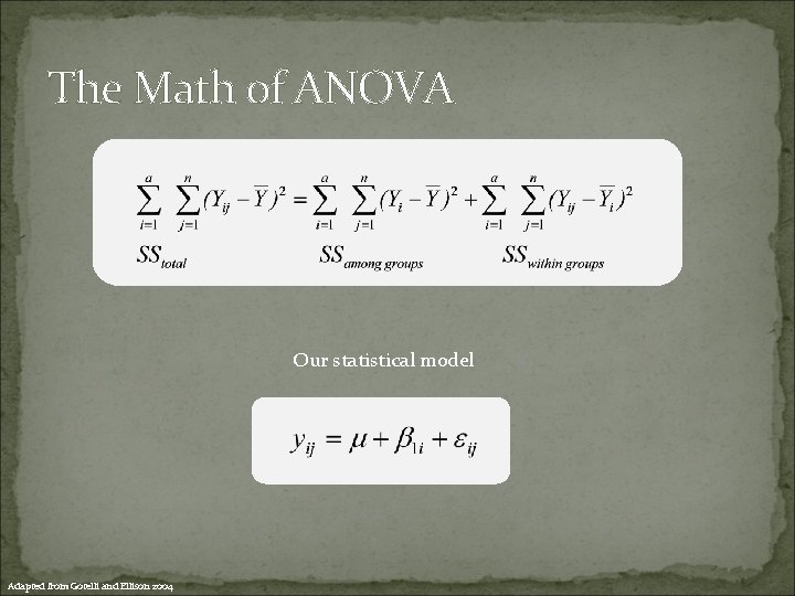
The Math of ANOVA Our statistical model Adapted from Gotelli and Ellison 2004

Where we're going �History of ANOVA �The Math of ANOVA �Bayes Theorem �Anatomy of Baysian ANOVA �Compare and Contrast! �Rumble in the Jungle: Advantages of Bayes �Real World 13: Genotype and Frequency Dependence in an invasive grass.
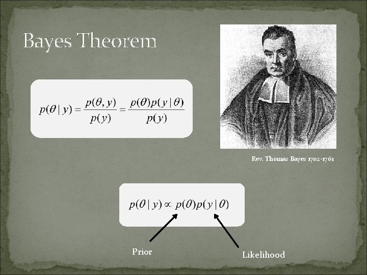
Bayes Theorem Rev. Thomas Bayes 1702 -1761 Prior Likelihood
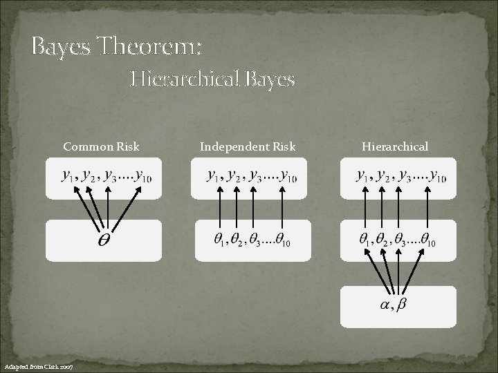
Bayes Theorem: Hierarchical Bayes Common Risk Adapted from Clark 2007 Independent Risk Hierarchical
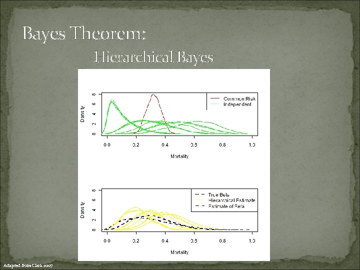
Bayes Theorem: Hierarchical Bayes Adapted from Clark 2007

Where we're going �History of ANOVA �The Math of ANOVA �Bayes Theorem �Anatomy of Baysian ANOVA �Compare and Contrast! �Rumble in the Jungle: Advantages of Bayes �Real World 13: Genotype and Frequency Dependence in an invasive grass.

Anatomy of Bayesian ANOVA or
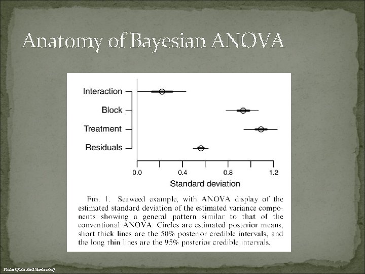
Anatomy of Bayesian ANOVA From Qian and Shen 2007
Where we're going �History of ANOVA �The Math of ANOVA �Bayes Theorem �Anatomy of Baysian ANOVA �Compare and Contrast! �Rumble in the Jungle: Advantages of Bayes �Real World 13: Genotype and Frequency Dependence in an invasive grass.
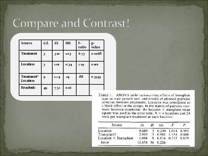
Compare and Contrast! Source d. f. SS MS Fratio pvalue Treatment 3 3. 10 1. 03 6. 73 0. 0068 Location 3 1. 01 0. 34 2. 19 0. 101 Treatment* Location 9 1. 24 . 14 . 88 0. 5543 Residuals 49 7. 52 0. 16
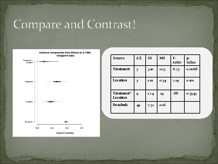
Compare and Contrast! Source d. f. SS MS Fratio pvalue Treatment 3 3. 10 1. 03 6. 73 0. 0068 Location 3 1. 01 0. 34 2. 19 0. 101 Treatment* Location 9 1. 24 . 14 . 88 0. 5543 Residuals 49 7. 52 0. 16
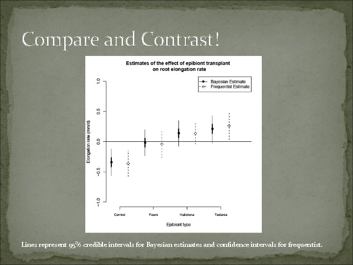
Compare and Contrast! Lines represent 95% credible intervals for Bayesian estimates and confidence intervals for frequentist.
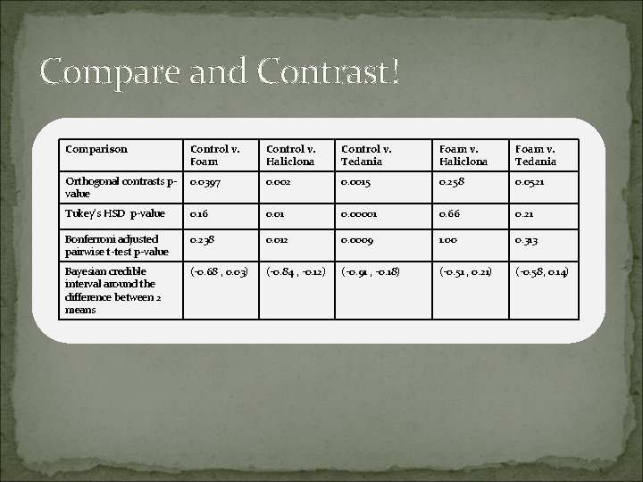
Compare and Contrast! Comparison Control v. Foam Control v. Haliclona Control v. Tedania Foam v. Haliclona Foam v. Tedania Orthogonal contrasts pvalue 0. 0397 0. 002 0. 0015 0. 258 0. 0521 Tukey’s HSD p-value 0. 16 0. 01 0. 00001 0. 66 0. 21 Bonferroni adjusted pairwise t-test p-value 0. 238 0. 012 0. 0009 1. 00 0. 313 Bayesian credible interval around the difference between 2 means (-0. 68 , 0. 03) (-0. 84 , -0. 12) (-0. 91 , -0. 18) (-0. 51 , 0. 21) (-0. 58, 0. 14)

Where we're going �History of ANOVA �The Math of ANOVA �Bayes Theorem �Anatomy of Baysian ANOVA �Compare and Contrast! �Rumble in the Jungle: Advantages of Bayes �Real World 13: Genotype and Frequency Dependence in an invasive grass.
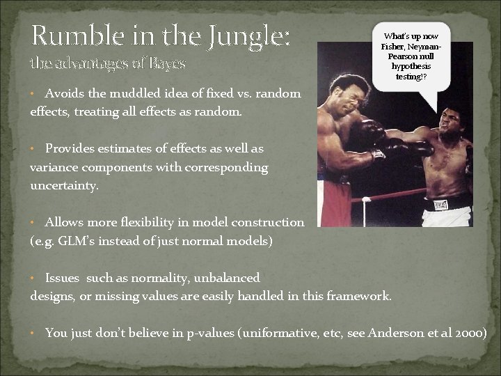
Rumble in the Jungle: the advantages of Bayes What’s up now Fisher, Neyman. Pearson null hypothesis testing!? • Avoids the muddled idea of fixed vs. random effects, treating all effects as random. • Provides estimates of effects as well as variance components with corresponding uncertainty. • Allows more flexibility in model construction (e. g. GLM’s instead of just normal models) • Issues such as normality, unbalanced designs, or missing values are easily handled in this framework. • You just don’t believe in p-values (uniformative, etc, see Anderson et al 2000)
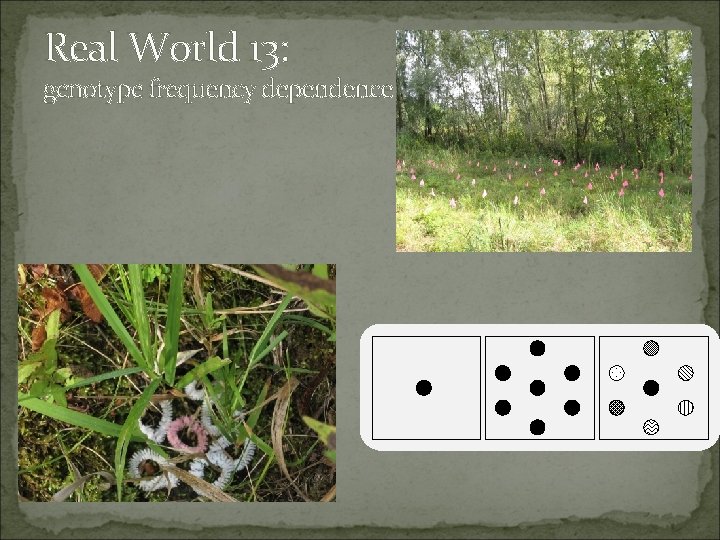
Real World 13: genotype frequency dependence
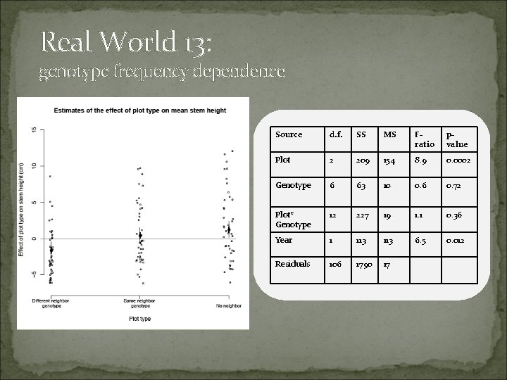
Real World 13: genotype frequency dependence Source d. f. SS MS Fratio pvalue Plot 2 209 154 8. 9 0. 0002 Genotype 6 63 10 0. 6 0. 72 Plot* Genotype 12 227 19 1. 1 0. 36 Year 1 113 6. 5 0. 012 Residuals 106 1790 17
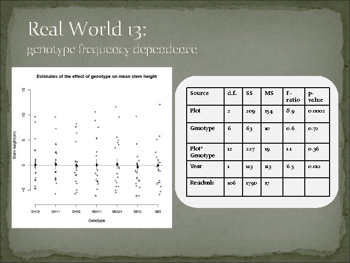
Real World 13: genotype frequency dependence Source d. f. SS MS Fratio pvalue Plot 2 209 154 8. 9 0. 0002 Genotype 6 63 10 0. 6 0. 72 Plot* Genotype 12 227 19 1. 1 0. 36 Year 1 113 6. 5 0. 012 Residuals 106 1790 17
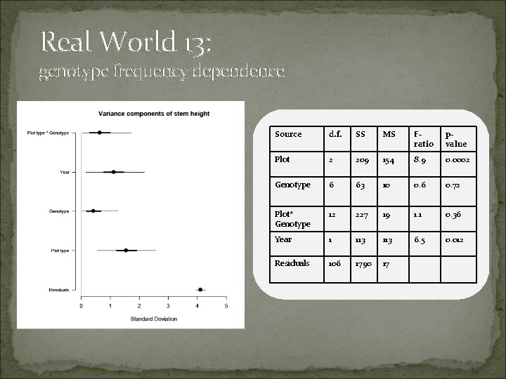
Real World 13: genotype frequency dependence Source d. f. SS MS Fratio pvalue Plot 2 209 154 8. 9 0. 0002 Genotype 6 63 10 0. 6 0. 72 Plot* Genotype 12 227 19 1. 1 0. 36 Year 1 113 6. 5 0. 012 Residuals 106 1790 17
![model { Thanks! Robin Collins Nick Gotelli for( i in 1: n){ y[i] ~ model { Thanks! Robin Collins Nick Gotelli for( i in 1: n){ y[i] ~](http://slidetodoc.com/presentation_image_h2/dfd45aa9cc3031b89f2dfd840e8b68f7/image-27.jpg)
model { Thanks! Robin Collins Nick Gotelli for( i in 1: n){ y[i] ~ dnorm(y. mu[i], tau. y) y. mu[i] <- mu + delta[plottype[i]] + gamma[studyyear[i]] + nu[gens[i]] + interact[plottype[i], gens[i]] } mu ~ dnorm(0, . 0001) tau. y <- pow(sigma. y, -2) sigma. y ~ dunif(0, 100) mu. adj <- mu + mean(delta[])+mean(gamma[]) +mean(nu[])+mean(interact[, ]) #compute for(i in e. y[i] s. y <- finite population standard deviation 1: n){ <- y[i] - y. mu[i]} sd(e. y[]) xi. d ~dnorm(0, tau. d. xi) tau. d. xi <- pow(prior. scale. d, -2) for(k in 1: n. plottype){ delta[k] ~ dnorm(mu. d, tau. delta) d. adj[k] <- delta[k] - mean(delta[]) for(z in 1: n. gens) { interact[k, z]~dnorm(mu. inter, tau. inter) } }
- Slides: 27